24 (2000) 21}38
E
$
cient gradualism in intertemporal portfolios
Ronald J. Balvers*, Douglas W. Mitchell
Department of Economics, West Virginia University, P.O. Box 6025, Morgantown WV 26506, USA
Received 15 February 1997; accepted 22 September 1998
Abstract
This paper examines intertemporal portfolio plans under autocorrelation in asset returns, and considers whether these plans conform to the common advice that risky assets be bought gradually and then held in decreasing amounts as the investment horizon approaches. Given elliptical returns, optimal portfolio plans with precommit-ment must be mean}variance e$cient. Then, for ARMA (1, 1) parameterizations with negative autocorrelation, the age e!ect (gradual diminishing of risky holdings as the horizon approaches) is con"rmed, as is dollar-cost averaging (gradual entry into the risky asset) for su$ciently distant horizons. For a numerically analyzed alternative bivariate returns process, only the age e!ect is con"rmed. ( 2000 Elsevier Science B.V. All rights reserved.
JEL classixcation: G11 (primary); D81, D91 (secondary)
Keywords: Intertemporal portfolio choice; Dollar-cost averaging; Age e!ects; Mean}
variance e$ciency; Mean reversion
1. Introduction
Investment advisors often advocate dollar-cost averaging when acquiring risky asset holdings, and increasing conservatism when approaching retirement. Dollar-cost averaging involves buying the risky asset gradually over several periods rather than all at once, as a way of intertemporally diversifying with respect to the purchase price. The alleged rationale for an age e!ect on optimal risky holdings is that a greater remaining time to the investment horizon allows
for greater gains from intertemporal diversi"cation in that a bad rate of return in one period may be o!set by a good rate in a later period.
Both of these types of intertemporal advice have proved di$cult to con"rm analytically, although several papers have made progress in this regard. Samuel-son (1989a) shows that age e!ects can arise under non-constant relative risk aversion.1Samuelson (1991) showed that the conventionally advised age e!ect arises when the risky asset has a two-point distribution and returns are nega-tively serially correlated. Bodie et al. (1992) showed that age e!ects arise when younger people have more#exibility in responding to portfolio realizations by altering labor supply. See also Samuelson (1989b, 1990) and Jagannathan and Kocherlakota (1996) for discussions of these issues. On the other hand, Roze!
(1994) showed that linear dollar-cost averaging is mean}variance ine$cient if returns are independent through time.
The present paper follows Roze!in considering the issue of mean}variance e$ciency, but allows for serial dependence of returns. Existence of serial correla-tion in rates of return has been carefully documented by Poterba and Summers (1988) and Fama and French (1988) who"nd that, for yearly observations of stock returns, rates of return are signi"cantly negatively autocorrelated. This phenomenon re#ects a process of&mean reversion'(or, more accurately, trend reversion) in stock prices.2
Like the recent papers of Roze! (1994), Ehrlich and Hamlen (1995), and others, we consider the precommitment (open-loop) case in which the portfolio sequence is locked in advance. This assumption is realistic since the costs of
1Speci"cally, he considers utility functions;"log(=!c) or;"(=!c)c/cfor constantc'0, which have decreasing relative risk aversion. He shows that, for given current wealth, someone with longer to go until the investment horizon would hold a larger share in the risky asset, under intertemporal independence of returns. However, his model also implies that as an individual moves through time and wealth grows, on average, faster than the riskfree rate of return, the optimal risky share grows. To get the conventional age e!ect in this regard, one would have to assume increasing relative risk aversion.
2It is important to realize that mean reversion in asset prices is not necessarily associated with market ine$ciency. Balvers et al. (1990) and Cecchetti et al. (1990) show for instance that, with rational decision making by representative agents, trend reversion in the business cycle implies mean reversion in asset prices. Further, Chen (1991), Ilmanen (1995), and others show that decreasing relative risk aversion by the representative consumer can lead to mean reversion.
The mean reversion results have been contested. For instance Kim et al. (1991) argue that the
gathering and assessing information and implementing plan changes exceed the bene"ts of doing so for many individuals. Further, many of the insights gener-ated here carry over to situations where this is not so, in which case additional complications are introduced through feedback.3
The nature of the time path of the risky investment in mean}variance e$cient plans is considered. With a zero riskfree rate and serial independence of returns, the optimal absolute risky investment is constant over time; Roze! 's (1994) demonstration of the ine$ciency of linear dollar-cost averaging emerges as a corollary of this result. With returns following an AR(1) process, the optimal absolute risky investment is constant except that it is lower (higher) in the"rst and last periods if the"rst-order serial correlation is negative (positive). For the negative"rst-order serial correlation case this con"rms the conventional wis-dom of dollar-cost averaging and decreased absolute and relative holdings of the risky asset as retirement approaches. For ARMA (1, 1) parameterizations giving negative autocorrelation of returns at all lags, the age e!ect obtains, and dollar-cost averaging also obtains if the horizon is su$ciently distant.4 For a more complicated bivariate returns process involving positive short-term and negative long-term autocorrelations, for which analytical results cannot be obtained, simulations reveal only a modi"ed age e!ect.
As we examine mean}variance e$cient portfolios, it is worth recalling the assumptions under which all expected utility maximizing portfolios are mean}variance e$cient. By Chamberlain (1983) and Owen and Rabinovitch (1983), mean}variance analysis is equivalent to expected utility analysis if and only if returns are jointly elliptically distributed (which permits bounded distri-butions as well as the joint normal), and by Nelson (1990) all expected utility maximizing portfolios are then mean}variance e$cient. Since in our context
3Balvers and Mitchell (1997) also consider portfolio choice under mean reversion but without precommitment. Tractability considerations stemming from the absence of precommitment limit the analysis to a single speci"c utility function, displaying constant absolute risk aversion, whereas the present paper obtains results that are independent of the utility function. Unfortunately, an e!ort to combine the approach of allowing portfolio response to current conditions with the approach here, of seeking e$cient conditions applicable to all utility functions, becomes intractable. In particular, applying Kritzmans (1990) linear investment rules to our analysis would result in the loss of ellipticality of portfolio return, a feature crucial to our approach. The approach of this paper and that of Balvers and Mitchell (1997) lead to similar results concerning the age e!ect: mean reversion in risky asset prices creates a diversi"cation motive for gradual decline of risky holdings as the horizon approaches.
returns are jointly elliptical, these results from the literature apply here. Note that all that needs to be assumed about the utility function is that it is increasing and concave, so that mean-standard deviation indi!erence curves are upward sloped and convex.
Investors with di!erent utility functions will choose di!erent mean}variance e$cient portfolios. Nevertheless, any property common to all e$cient portfolios will be common to the optimal portfolios of all investors. The properties common to all e$cient portfolios are found by characterizing all such portfolios as minimizing the variance of"nal wealth contingent on some given level of expected "nal wealth, and noting what features of the e$cient portfolios are independent of the given expected wealth level. Because we focus on features common to all e$cient portfolios, an important strength of our analysis is that, given our assumptions of precommitment and elliptical returns,the results apply to all upward sloped, concave utility functions, not just to some speci"c utility function.
Section 2 analyzes the intertemporal mean}variance e$cient frontier that applies under all dynamic processes. Section 3 presents our main result: the various conditions under which dollar-cost averaging and age e!ects are or are not optimal under an ARMA (1, 1) process generating excess returns. Section 4 numerically considers an alternative, richer bivariate process, and Section 5 concludes.
2. Deriving e7cient time paths of the risky investment
In the¹-period problem,"nal wealth =
Tat the end of period ¹ is given by
=
T"=0(1#r&)T# T + t/1
w
txt, wt,At(1#r&)T~t, (1)
where=
0is initial wealth inherited from the end of period 0,xtrepresents the excess return of the risky asset over the riskless asset, andr
&is the riskless rate of
return. A
t represents the absolute amount invested in the risky asset at the beginning of time periodt; w
tis the future value of the wealth invested in the risky asset.
of using that information to devise and implement changes in the portfolio plan.5
The precommitment strategy at time 0 consists of jointly choosing thew tfor allt(t"1,2,¹) as of the beginning of period 1, based on knowledge of=0and
r
0. In any period t, wealth=t~1is inherited from the previous period and is invested according to the precommitted strategy. Then, during period t, the riskfree returnr
&and the excess returnxtare realized, resulting in end-of-period wealth =
t. Note that if the rates of return on the risky asset in the various periods are jointly elliptically distributed, as we will assume, then by Eq. (1)"nal wealth is elliptically distributed, so the conditions of Chamberlain (1983), Owen and Rabinovitch (1983), and Nelson (1990) for mean}variance analysis to be equivalent to expected utility analysis are met.
The optimal time path of w
t will clearly depend in part on the time-zero expectation of the risky return path. For example, if x
0is above its long-run mean value and if the dynamic process is monotonically mean-reverting, then
E
0x5will be a declining function of time; in this case the fact thatE0x5is highest
in the early periods obviously will impart a tendency for the risky asset to be held more in the early periods. Conversely, ifx
0is less than its long-run mean, the risky asset will be relatively unattractive in the early periods. This e!ect of the expected risky rate of return is not what we wish to investigate here; instead, we wish to focus on portfolio e!ects arising from the proximity of the beginning or the end of the sequence of investment periods. Thus we assume that the observed values at the end of period 0 of all variables equal their long-run means, implying that the mean risky rate of return conditional on information at time 0 is constant through time, i.e.,E0x
t"xN for allt. From Eq. (1) the mean and variance of=
T, conditional on all information about the dynamic returns process available at the end of time 0, are
E
0=T"=0(1#r&)T#(w@n)xN, (2)
p2WT"w@<w, (3) wherexN,E
0xq'0 (independent ofq),w,[w1,2,wT]@is the vector of future values of successive absolute investments in the risky asset,nis a¹]1 vector of ones, and <is a¹]¹positive-de"nite conditional covariance matrix withs,
qelement cov
0(rs,rq) . Thus the structure of<depends on the dynamic process generating the returns. The problem now is to"nd the intertemporal portfolio
vectorwthat minimizesp2
WTsubject toE0=T"k.6The Lagrangian is
¸"w@<w!2t(w@n!B), (4) whereB,[k!=
0(1#r&)T]/xN, and where 2tis the Lagrange multiplier. The "rst-order conditions are the constraint and
<w!tn"0, (5)
implying
w*"t*<~1n. (6)
t*is found by using Eq. (6) in the constraint:
t*"B/(n@<~1n). (7) The denominator in Eq. (7) is positive because<, and hence<~1, are positive de"nite. Thust*'0 providedB'0}i.e., providedk'=
0(1#r&)T(i.e. the
mean of "nal wealth is parametrically set above the wealth which could be achieved by a sequence of riskfree portfolios). We limit our focus to values of
ksuch thatB'0, sot*'0.
Eq. (6) shows the important role of the inverse covariance matrix; such a role is routine in mean}variance portfolio analysis. This equation implies that the future value of the optimal absolute risky investment in periodtis proportional to the tth row sum of the inverse covariance matrix. An important aspect of what follows will be to analyze the particular form that these row sums take under the dynamic excess returns processes to be speci"ed in what follows. The row sums, and hence the time pro"le of the optimal portfolio, will depend in a complicated way on the dynamic process speci"ed and its speci"c parameter values.
It will be convenient in what follows to analyze the time pro"le of e$cient portfolios in terms of s
t, the risky share of baseline wealth. De"ne baseline wealth at the start of periodtas=
0(1#r&)t~1; this is what wealth would be if all
previous portfolios had been invested entirely in the riskfree asset. Then:
s t"
A t =
0(1#r&)t~1
"A
t(1#r&)T~t=~10 (1#r&)1~T
"w
t=~10 (1#r&)1~T. (8)
This shows thats
tandwtare proportional to each other so that the nature of the time path ofs
tis the same as that ofwt.
6The e$cient locus for this¹-period problem is linear in (E=
3. Closed-form portfolio paths under an ARMA(1, 1) returns process
In this section we assume that the excess return follows a general ARMA (1, 1) process:
x
t"oxt~1#(1!o)b!det~1#et. (9) Herebis a positive constant representing the long-run mean value of the excess rate of return, and we assumed3[!1, 1] ando3(!1, 1). The processMetNis elliptically distributed white noise. For this process"rst-order autocorrelation has the sign ofo!dwhile higher-order autocorrelations (of orderk) have the sign ofok~1(o!d). Partial autocorrelations have the sign ofdk~1(o!d).
For process (9) we obtain the following analytical results for the time pro"le of e$cient portfolio paths:
¹heorem.Assume the ARMA(1, 1)process for the excess return as in Eq. (9).¹hen for the mean}variance e.cient precommitment portfolio plan:
(a) Ifo"d3(!1, 1),s
tis constant over time. (b) Ifd"0and!1(o(0,s
tis constant for periods2through¹!1,but is lower in periods1and¹.
(c) Ifd"0and0(o(1,s
tis constant for periods2through¹!1,but is high -er in p-eriods1and¹.
(d) Ifd"1and!1(o(1,the path of s
qis characterized by st'st`1for t" 1,2,¹!1.
(e) If0(d(1and!1(o(d,then for t((¹#1)/2we have s
t~1Nst,while for t5(¹#1)/2we have s
t'st`1.
(f ) If0(d(1andd(o(1,then for t4(¹#1)/2we have s
t~1'st,while for t'(¹#1)/2we have s
tNst`1.
Proof. Given Eq. (9), the appendix derives the intertemporal covariance matrix
<conditional on information at time 0:
<
sq/p2e"
G
oq~s~1[o(<
ss/p2e)!d] fors(q, 1#(o!d)2(1!o2(s~1))/(1!o2) fors"q,
os~q~1[o(<
qq/p2e)!d] fors'q.
(10)
De"ningz
t"wt(p2e/t), Eq. (5) implies that
T + q/1
(<
tq/p2e)zq"1 fort"1,2,¹. (11) Appendix A shows that for the case of dO1, Eqs. (10) and (11) yield the following solution forz
to the risky shares
tof baseline wealth:
z t"
1
(1!d)2[(1!o)2#(o!d) (1!o)dT~t#
(1!do)(o!d) 1#d dt~1
#(o!d)2
1#d d2T~t]. (12)
Ford"1, Appendix A shows that the path ofMz
tNis characterized by z
t"zt`1#(1!o)2t, (13) withz
T"o#(1!o)¹.
The proof of (a) follows from inspection of Eq. (12). For cases (b) and (c), with
d"0, (12) implies
z t"
G
(1!o)2 fort"2,2,¹!1, (1!o)2#o fort"1,
(1!o)2#o(1!o) fort"¹,
(14)
where fort"1 and¹use has been made of the identity 00,1. Cases (b) and (c) are proven by inspection of Eq. (14). Case (d) is proven by inspection of Eq. (13). For cases (e) and (f), with 0(d(1, de"ne the right-hand side of Eq. (12) as a functionfof a continuous variablet, so the discrete sequenceMz
tNcomprises a discrete set of values generated by that function. Then we can di!erentiate the right side of Eq. (12) with respect tot:
df/dt"!(lnd)(o!d)dT~t
(1!d)2(1#d) [(1#d)(1!o)!(1!do)d2t~1~T
#(o!d)dT]. (15)
Since 0(d(1 in the cases under consideration, lndexists and is negative. Thus
sgn df/dt"sgn(o!d)[(1#d)(1!o)!(1!do)d2t~1~T#(o!d)dT](16) or, equivalently,
sgn df/dt"sgn[(o!d)2(dT!1)!(o!d)(1!do)(d2t~1~T!1)]. (17) Noting that with 0(d(1 expressions of the form dg are N 1, as g~0, we have df/dt(0 if (2t!1!¹)50 and o(d; additionally df/dt(0 if (2t!1!¹)40 ando'd. Otherwise df/dtl0. The cases with df/dt(0 imply
z
t'zt`1 since zt"f(t) by Eq. (12), and thus imply wt'wt`1 and therefore
s
t'st`1; this proves cases (e) and (f ). QED. Note that if, for example,s
tand hencewtstays constant over time as in part (a) of the theorem so thatA
A
t/=ton average declines over time since=tis expected to grow faster than the rater
&if positive amounts are invested in the risky asset. Therefore the
conven-tional age e!ect of a declining risky share obtains even with i.i.d. returns. The results of the theorem are in terms of the risky shares
tof baseline wealth, whereas discussions of dollar-cost averaging are normally in terms of the absolute risky amountA
t. These di!er whenr&O0. In order to disentangle this
e!ect of nonzeror
&from the e!ect of autocorrelated returns, in the exposition
which follows we will consider the case in whichr
&"0. Ifr&'0, an upward tilt
is imparted on the time path ofA
trelative to that ofst. Also note that Roze!'s (1994) result, that dollar-cost averaging of absolute risky holdings is mean}
variance ine$cient when returns are intertemporally independent, emerges as a corollary of case (a) wheno"0"dandr
&"0.
The theorem shows, foro(dwith d3[0, 1], that the risky asset holdings decline as the horizon approaches, in absolute terms and therefore also (because on average wealth grows over time) relative to wealth. Dollar-cost averaging always obtains if o(d"0. Now consider dollar-cost averaging under the parameter conditions of case (e):d3(0, 1) ando(d. The theorem indicates that, in contrast to the situation for latert, fort((¹#1)/2 the slope of the time path is ambiguous in general; however, for ¹PRone can see from Eq. (12) that
z
2'z1 so that dollar-cost averaging again obtains. Eq. (12) also reveals that a&turnpike'result holds. Namely, for¹PRthe time that the optimal solution,
z
t, spends close to the turnpike outcome, [(1!o)/(1!d)]2, also goes to in"nity.7
Interestingly, ifd"1, case (d), dollar-cost averaging is never optimal and no turnpike result obtains. On the other hand, consider the case of negative partial autocorrelation at all lags }which is the empirically relevant case for annual data according to the results of Fama and French (1988) and Poterba and Summers (1988). Since partial autocorrelation of order k has the sign of
dk~1(o!d), such negative partial autocorrelation requires 0(d and o(d; thus by case (e) both dollar-cost averaging (for large enough¹) and the age e!ect obtain.
Why does negative partial autocorrelation in the returns typically imply the inverse U-shape over time for the absolute amount invested? The answer lies in the analogy with a standard static mean}variance portfolio problem: consider the investment opportunity for each year as a di!erent asset. The main di!erence then is that here the correlation between the assets is clearly speci"ed}assets
7To prove this based on Eq. (12) consider three strictly positive,"nite constants:a,b, andc. De"neu"a#b#c. Setq1"(a/u)¹andq2"[(a#b)/u]¹and sett
iequal to the integer closest
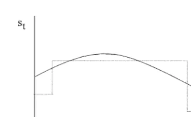
Fig. 1. Risky investment over time with negative autocorrelation.
closer together in time have stronger negative partial autocorrelation. It is the
partialautocorrelation which determines the marginal risk impact (that is, the contribution to overall portfolio risk) of such a time-speci"c asset. Accordingly, assets in the early investment periods have fewer assets that are strongly negatively partially correlated with them to o!set their risk and thus are less popular and the same is true for assets close to the investment horizon. Assets towards the middle of the investment sequence are the most &diversi"ed', and thus are acquired in larger quantity. In contrast, in the case of independent returns as considered by Roze!(1994)}case (a)}the position of the asset in time is irrelevant, so a#at pro"le of risky holdings results.
Fig. 1 displays the typical pattern of the risky share of baseline wealth under mean reversion (negatively autocorrelated returns, which in our context implies negative partial autocorrelation at all lags). Assuming the investment horizon is far enough away, case (e) yields the inverse U-shape as indicated by the bold line. The shape is not symmetric. The reason is that due to the precommitment assumption risk increases over time: the conditional variance of the risky return rises as time is further from the decision period. This by itself would cause the risky share of baseline wealth to fall over time and explains why dollar-cost averaging may not occur, even in case (e), when the investment horizon is near. The dotted line in Fig. 1 displays the AR(1) case, case (b), which has partial autocorrelation that is negative at order one and zero at higher orders. Thus negative partial autocorrelation is only with the nearest asset, which explains the pattern; the increasing conditional return variance again causes asymmetry, with more risky investment in the"rst period than in the last.
4. A numerical example for a bivariate returns process
as pointed out by Lo and Wang (1995), returns in high-frequency data are positively autocorrelated at short lags but negatively autocorrelated at longer lags. Consequently, in this section we consider a process which is capable of generating such a pattern. Speci"cally, we employ a discrete-time version of the bivariate Ornstein}Uhlenbeck process used by Lo and Wang. While this pro-cess will not permit us to obtain analytical results comparable to those in the theorem for the ARMA(1, 1) process, we do present numerical results based on calibrating the parameters of the process to U.S. post-war data.
Clearly the presence of both positive and negative autocorrelations will produce con#icting e!ects on the direction of change of portfolio shares over time, since negative autocorrelations create a risk-reducing role for time
diversi-"cation while positive autocorrelations do the reverse. Intuitively, we expect that when many periods remain until the horizon the negative long-lag auto-correlations will predominate and, as discussed previously, a conventional age e!ect in which risky investment declines over time will occur. However, when the horizon is very near, the positive short-lag autocorrelations will predomi-nate, causing a reverse age e!ect.
All of the equations in Section 2, culminating in Eq. (8) for the risky share of baseline wealth, still apply. Instead of Eq. (9) of Section 3, we now assume the following bivariate process for deviationsp
tof logged stock prices (with reinves-ted dividends) from trend
p
t"j(pt~1!ht~1)#et, (18) h
t"oht~1#gt. (19) Heregandeare elliptically distributed white noise, andhis a latent variable. Then the excess return is given by
x
t"pt!pt~1#h!r&, (20)
wherehis the slope of the logged stock price trend line. Note that the process in Eqs. (18)}(20) is di!erent from, but not a generalization of, the ARMA(1, 1) process in the previous section.
We will use the unconditional autocovariance function to calibrate the stochastic process of Eqs. (18)}(20) to U.S. data. This autocovariance function, withkdenoting the lag, is
c(0)" 2 1#j
A
j2p2 g
(1!jo)(1#o)#p2e
B
, (21a)c(k)" j2
(1!oj)(j!o)
CA
1!o1#o
B
ok!A
1!j1#j
B
jkD
p2g!A
(1!j)j(1#j)
B
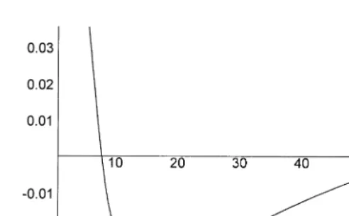
jkp2eFig. 2. The unconditional autocorrelation function.
Following Lo and Wang (1995), we perform the calibration by using Eqs. (21a) and (21b) fork"0, 1, 5, 25, but using monthly instead of daily data. Our data consist of monthly excess returns based on the CRSP equal-weighted returns index for 1947.1}1996.12. From these data we compute c(k) for the indicated
k-values, and substitute thesec(k) values into Eqs. (21a) and (21b) for each of
k"0, 1, 5, 25. These values are, respectively, 26.331, 4.134, 0.737, and!0.632. This substitution yields four equations in the four unknownsj,o,p2
e,p2g, which we solve numerically in order to match exactly the four moments. The solution is Mj,o,p2
e,p2gN"M0.946, 0.801, 19.596, 2.927N. The resulting autocorrelation function fork"0, 1, 2,2, shown in Fig. 2, is positive at short lags and negative at longer lags.
To compute the e$cient path of the risky share s
t of baseline wealth, by Eqs. (8) and (6) we need the row sums of the inverse of the conditional autocovariance matrix. Therefore, we use the above numerical parameter values in the following conditional autocovariance function, where we de"nec
t(k) as the covariance betweenx
tandxt~kconditional on realizations of all variables through time 0:
c t(0)"
p2 gj2 (j!o)2
A
(1!j)
1#j[1!j2(t~1)]# (1!o)
1#o [1!o2(t~1)] !2(1!j)(1!o)
1!jo [1!(jo)t~1]
B
# p2e
1#j[2!(1!j)j2(t~1)], (22a)
c
t(k)"p2g
A
t~1 + j/k
b
jbj~k
B
!p2eA
(1!j)(1#j2(t~k)~1)jk~1
Fig. 3. Normalized risky share of baseline wealth.
where
b j"
j
j!o[jj~1(1!j)!oj~1(1!o)].
Using Eqs. (22a) and (22b) along with Eqs. (6) and (8), we obtain the time path of the risky shares
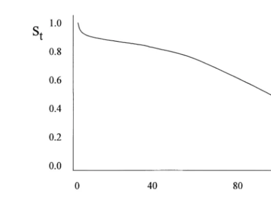
tof baseline wealth. Since this path depends on the row sums of the¹]¹matrix<~1, it depends on the time horizon¹. A horizon of"ve or ten years would be representative for many individuals saving for their chil-dren's college education, for a house purchase, or for retirement. Fig. 3 depicts this path for a ten-year horizon,¹"120. Because the magnitude (though not the pattern) of the s
t values depends on the speci"c location chosen on the e$cient frontier, which in turn depends on the utility function, we normalize in Fig. 3 by setting s
1"1. As our earlier intuition suggested, this time path is generally downward sloped except for an upturn near the horizon; these features are due to the predominance of the negative long-lag autocorrelations when substantial investment time remains, and of the positive short-lag autocorrela-tions as the horizon gets very near. Hence, the dynamic process of the current section, with the parameter values"tted to U.S. data, demonstrates the conven-tional age e!ect with a slight modi"cation.
only two qualitative patterns ofs
t: that shown in Fig. 3, and a pattern like that in Fig. 3 but without the upturn at the end. Dollar-cost averaging never occurs. To get a feel for why it does not, note that a special case of the bivariate process of this section coincides with a special case of our earlier ARMA(1, 1) process for which the theorem showed that dollar-cost averaging cannot occur. Speci"cally, whenp
g"0 the bivariate model collapses to the ARMA(1, 1) model withd"1; part (d) of the theorem precluded dollar-cost averaging in this case.
This section has explored the implications of adopting a more complicated process allowing the realistic feature of positive short-lag and negative longer-lag autocorrelations in excess returns. The results reinforce the conventional notion of age e!ects in long-horizon investment plans.
5. Conclusion
This paper has considered the question of whether mean}variance e$cient open-loop portfolio plans in the presence of mean reversion in risky asset prices conform to the commonly given advice that risky assets should be bought gradually and then held in decreasing quantities as the investment horizon approaches. The paper showed the conditions under which mean}variance e$ciency is relevant, and demonstrated analytically that relative holdings of the risky asset should indeed be diminished as retirement approaches if returns are ARMA (1, 1) and are negatively correlated at all lags; in this case dollar-cost averaging as the risky asset is"rst acquired is also optimal, provided the horizon is su$ciently distant. The conventional age e!ect is also substantially con"rmed, numerically, for more complicated dynamics in which returns autocorrelations are positive at short lags and negative at longer lags. These results suggest that investment advisors implicitly predicate their recommendations on the assump-tion that asset prices are indeed mean reverting.
It should be noted that in practice, when portfolio plans are formulated, the excess return may not be at its long-run average value. If the excess return is initially above its long-run mean, for instance, mean reversion would impart a downward tilt to the time path of risky asset holdings. Thus it can be said that the optimal investment strategy should depend on the phase of the&asset return cycle'. An interesting area for future research would be to seek evidence of such a phase-of-cycle e!ect in investment advice.
the paper focused on two classes of returns processes, our approach of analyzing the mean}variance e$cient locus is valid in general, and can be used to explore the implications of any returns process analytically or numerically. Finally, another potential avenue for future research would be to try to extend the results to the context of n-asset portfolios. Such an extension would be di$cult, however, in that it would involve diversi"cation in two dimensions } cross-sectionally and intertemporally}rather than just one.
Acknowledgements
The authors thank the anonymous referee for helpful comments.
Appendix A.
A.1. Derivation of Eq. (10)
To derive Eq. (10), recursively solve for Eq. (9) for realizations between times 0 andt, producing
Take conditional expectations in Eq. (A.1) for given information at time 0 and use the de"nition of covariance, to produce
<
Now, without loss of generality, assume thatt5s. Keep in mind that thee
tare serially uncorrelated. Then, fort's,
Fort"s, it follows from Eq. (A.2) that yields, with the help of Eq. (10),
1!o"!dz
Fort"1, Eqs. (10) and (11) produce
1"z
Denoting the successive right-hand sides of Eqs. (A.7), (A.8),2asyt(t"1, 2, 3, 2,¹!1), continuing this process yields
y
Delaying Eq. (A.10) by one period and adding this too times (A.10) yields
y
t~1!oyt"zt~1!dzt. Applying the recursive formula forytproduces (1!do)y
t!o(1!o)"zt!dzt`1, t"1,2,¹!1. (A.11) To obtain an expression for time¹as well, take Eq. (A.6) fort"¹!1:
1!o"!dz
To "nd z
T, add d times (A.11) evaluated at ¹!1 to Eq. (A.12) and use y
T"dyT~1#1!oto yieldzT"yT. Consider"rst the case ofdO1. ThenyT is obtained by solving the di!erence equation y
t"dyt~1#1!o, y1"1, producing
y t"
1!o#(o!d)dt~1
1!d , t"1,2,¹ (A.13)
and then evaluating at¹.
Solving Eq. (A.11) using Eq. (A.13) gives
z
t"dT~tzT#
A
1!o1!d
B
2
(1!dT~t) #(1!do)(o!d)
(1!d2)(1!d)dt~1[1!d2(T~t)]. (A.14)
Employing the fact thatz
T"yT, Eq. (A.13) evaluated at time¹and substituted into Eq. (A.14) produces Eq. (12) in the text.
A.3. Derivation of Eq. (13)
As Eqs. (A.13) and (A.14) are not valid ford"1, we obtain theMz
tNfor this case as follows: (A.11) withd"1 gives
z
t`1"zt#o(1!o)!(1!o)xt. (A.15) The processy
t"yt~1#(1!o) withy1"1 has the solutionyt"o#(1!o)t; using this in Eq. (A.15) gives
z
t`1"zt!(1!o)2t. (A.16) To obtain the terminal valuez
T, we use Eq. (A.15) att"¹!1 to give (d!o)y
T~1!o(1!o)!zT~1#zT"0 (A.17) and Eq. (A.12) withd"1 gives
(1!o)#z
T~1!(2!o)zT"0. (A.18) Adding Eq. (A.17) to Eq. (A.18) and dividing by (1!o) gives
y
T~1#(1!o)"zT. (A.19)
Since the left side of Eq. (A.19) equalsy
T, which equalso#(1!o)¹, we have z
References
Balvers, R.J., Cosimano, T.F., McDonald, B., 1990. Predicting stock returns in an e$cient market. Journal of Finance 45, 1109}1128.
Balvers, R.J., Mitchell, D.W., 1997. Autocorrelated returns and optimal intertemporal portfolio choice. Management Science 43, 1537}1551.
Bodie, Z., Merton, R.C., Samuelson, W.F., 1992. Labor Supply#exibility and portfolio choice in a life cycle model. Journal of Economic Dynamics and Control 16, 427}450.
Cecchetti, S., Lam, P., Mark, N., 1990. Mean reversion in equilibrium asset prices. American Economic Review 80, 398}418.
Chamberlain, G., 1983. A characterization of the distributions that imply mean}variance utility functions. Journal of Economic Theory 29, 185}201.
Chen, N., 1991. Financial investment opportunities and the macroeconomy. Journal of Finance 46, 529}554.
Fama, E., French, K., 1988. Permanent and temporary components of stock prices. Journal of Political Economy 96, 246}273.
Ilmanen, A., 1995. Time-varying expected returns in international bond markets. Journal of Finance 50, 481}506.
Jagannathan, R., Kocherlakota, N., 1996. Why should older people invest less in stocks than younger people? Federal Reserve Bank of Minneapolis Quarterly Review 11-23.
Kim, M., Nelson, C., Startz, R., 1991. Mean reversion in stock prices? A reappraisal of the empirical evidence. Review of Economic Studies 58, 515}528.
Kritzman, M.P., 1990. Asset Allocation for Institutional Portfolios. Irwin Publ. Co, Homewood, IL. Lo, A.W., Wang, J., 1995. Implementing option pricing models when asset returns are predictable.
Journal of Finance 50, 87}129.
Meyer, J., 1987. Two-moment decision models and expected utility. American Economic Review 77, 421}430.
Nelson, C.H., 1990. Two-moment decision models, portfolio choice, and elliptical symmetry, Working paper, Department of Agricultural Economics, University of Illinois.
Owen, J., Rabinovitch, R., 1983. On the class of elliptical distributions and their applications to the theory of portfolio choice. Journal of Finance 38, 745}752.
Poterba, J., Summers, L., 1988. Mean reversion in stock prices: Evidence and implications. Journal of Financial Economics 22, 27}59.
Richardson, M., Stock, J.H., 1989. Drawing inferences from statistics based on multiyear asset returns. Journal of Financial Economics 25, 323}348.
Roze!, M.S., 1994. Lump-sum investing versus dollar-averaging. Journal of Portfolio Management 20, 45}50.
Samuelson, P.A., 1989a. A Case at Last for Age-Phased Reduction in Equity. National Academy of Sciences, USA, vol. 86, pp. 9048}9051.
Samuelson, P.A., 1989b. The judgement of economic science on rational portfolio management: Indexing, timing and long-horizon e!ects. Journal of Portfolio Management 15, 4}12. Samuelson, P.A., 1990. Asset allocation could be dangerous to your health. Journal of Portfolio
Management 16, 5}8.
Samuelson, P.A., 1991. Long-run risk tolerance when equity returns are mean regressing: Pseudoparadoxes and vindication of &businessman's risk'. In: Brainard, W., Nordhaus, W., Watts, H. (Eds.), Money, Macroeconomics, and Economic Policy: Essays in Honor of James Tobin. MIT Press, Cambridge ch. 7.