Rates upon Duration and Convexity of Risky Debt
Vance P. Lesseig
UNIVERSITY OFTENNESSEE ATCHATTANOOGA
Duane Stock
UNIVERSITY OFOKLAHOMA
Early analysis of duration ignored default risk. Of course, many debt convexity states simply that the greater the convexity, the more valuable the bond (Grantier, 1988). This is logical because
instruments have at least some potential for default. Recent analyses have
partially filled this void. In our more complete model, we consider that convexity essentially compares the positive price movement from a decline in interest rates to the negative price movement
the default potential of debt issued by many firms is at least partially
dependent upon interest rates. The lower the credit quality of the debt, from an increase in rates. The greater the convexity, the greater the upside potential compared to the downside potential from
the more important this relation becomes. We explore the duration and
convexity of both senior and junior debt. We find that the relation of interest rate movements. Thus many portfolio strategies en-couraged maximizing convexity,ceteris paribus, although the
asset values to interest rates affects both duration and convexity of debt.
Additionally, the effect of this relationship on convexity is significantly effectiveness of this has been questioned [see Schnabel (1990) and Kahn and Lochoff (1990)]. Notwithstanding some of the
affected by the shape of the term structure. J BUSN RES2000. 49.289–
301. 2000 Elsevier Science Inc. All rights reserved. criticisms, convexity is still considered an important character-istic of a bond. Therefore it is important to consider the impact of the relation between interest rates and asset value upon both the duration and convexity of a firm’s debt.
The purpose of this research is to analyze the asset value
B
ecause of its importance in bond price volatilitymea-effect upon duration and convexity. That is, we go beyond surement, bond portfolio immunization, and financial
the work of other models by including and focusing upon institution management, duration has been analyzed a
the relation between interest rates and asset value. This is great deal. Most, but not all analysis has been of
default-done by utilizing a binomial model for pricing debt and then free debt. Fisher and Weil (1971), among others, analyzed
computing duration and convexity for bonds with default immunization under a non-flat term structure. Bierwag (1977)
risk. We include analysis of both senior and subordinated was one of the first to provide a rigorous analysis of duration
debt. The greater riskiness of subordinated (junior) debt en-for various types of changes in term structures. More recently,
hances the effects we observe for senior debt. Our model Chambers, Carleton, and McEnally (1988), advocated the use
shows that junior duration and convexity are more sensitive of duration vectors to improve immunization performance
to various parameters than senior debt. and Stock and Simonson (1988) examined the duration of
Our results indicate that an increasingly negative relation amortizing instruments. Prisman and Shores (1988) analyzed
between asset value and interest rates causes both duration and duration measures for specific term structure estimations. In
convexity to increase, while an increasingly positive relation their modelling of risky debt, Longstaff and Schwartz (1995)
causes both to decrease. Increasing the default risk of the maintain that the duration of risky debt may decline as it
issuer causes this effect to be enhanced. When junior debt is reaches maturity and depends on the correlation of assets with
considered, the risk and the sensitivity become even more interest rates.
important. For instance, we show that convexity values can Although convexity has attracted less attention, it is also
vary by as much as 50% by simply altering the issuer’s sensitiv-an importsensitiv-ant tool of bond sensitiv-analysis. Some early literature on
ity to interest rates. Additionally, in our model, this effect is directly affected by the shape of the term structure. We find Address correspondence to Dr. D. Stock, Finance Division, 205-A Adams Hall, that the steeper the slope of the term structure the greater University of Oklahoma, Norman, OK 73019. Tel.: (405) 325-5591; fax: (405)
325-1957; E-mail: [email protected] the impact of asset interest-rate sensitivity. A flat structure
Journal of Business Research 49, 289–301 (2000)
2000 Elsevier Science Inc. All rights reserved. ISSN 0148-2963/00/$–see front matter
substantially reduces the impact of this asset sensitivity and assets depends on default risk. More specifically, duration is a weighted average of the firm’s asset duration and duration provides duration and convexity measures quite close to
risk-less measures. of a risk free pure discount bond. (The weights are the elasticity of a default risky bond with respect to firm assets and the One of the more interesting findings is that default risk
alone does not have a strong effect on duration and convexity elasticity of a default risky bond with respect to a risk free bond.) Nawalkha (1996) shows that the duration of a risky in the absence of asset sensitivity. Even with high leverage
and volatility and using junior debt, if the issuer’s assets are bond must then be something between that of the duration of assets and that of the pure discount bond. He also finds insensitive to interest rates the debt displays duration and
convexity similar to that of riskless debt. This result reinforces that if asset duration is positive, Chance’s (1990) measure of duration is biased downward. Furthermore, if asset duration the importance of the interest-rate sensitivity of an issuer’s
assets on the performance of debt. However, in cases where is greater than bond maturity, then duration of the risky bond is greater than maturity. However, Nawalkha (1996) does not assets are interest-rate sensitive, greater leverage and volatility
have a quite strong impact on the difference between senior consider duration of junior versus senior debt nor does he consider the convexity of risky debt or the impact of term and junior duration and convexity.
structure shape upon duration and convexity. Furthermore, The rest of the article is organized as follows. The next
he includes no empirical analysis of his theory (as we do in section provides a discussion of the important attributes of
Appendix B). duration and convexity as well as a discussion of interest-rate
To compute duration our approach follows that of Garman sensitivity. The third section describes the model we have
(1985) where duration will be computed from the following developed, and the fourth section presents hypotheses
regard-[Eq. (1)]: ing duration and convexity with respect to our model. The
fifth section discusses the results and compares them to those
hypothesized. The last section concludes the article. D5DP Dr
1 Po
. (1)
HereDP is the price change due to the shift in rates, Dr is
Duration and Convexity
the size of the parallel term structure shift, and Pois the initial
price of the bond. In our simulation Dr will be a five basis Duration is often defined as the weighted average timing of
point parallel shift over the entire term structure. Convexity cash flows; it is frequently developed from the first derivative
is computed with Equation (2). of the price function (P) with respect to yield (y) and thus
measures the sensitivity of a security’s value to changes in
yield. Convexity compares the relative impact of both a posi- C5P1 1P222Po (Dr)2
1 Po
(2) tive and negative shift in yields on bond value. The functional
forms of both duration and convexity are derived from a where P1is the price after a positive shift in the term structure, Taylor series expansion of the price equation. Duration, (]P/ P
2is the price after a negative shift in the term structure, and
]y)/P, is represented by the first term and convexity, (]2P/]y2)/
Pois the original price of the bond.
P, by the second. Because duration measures price sensitivity, Because we model asset value as a function of interest rates, convexity measures the change in that sensitivity. The con- both duration and convexity measures will be influenced by cepts arise from the tradeoff between prices and yields of the asset sensitivity to interest rates. The importance of this bonds as shown in Figure 1. The general shape is convex and relation is perhaps most apparent when considering debt is-the Taylor expansion provides a close approximation to is-the sued by financial institutions whose assets are dominated by shape of the curve. rate-sensitive instruments. For industrial firms the issue of The pricing of zero coupon bonds is a simple equation, correlation is not as often recognized but can be significant P5F[e2yT], where F is the face value, y is the yield, and T for the value of a firm’s debt. Consider industries such as
is the time to maturity. From this equation duration is equal automobiles and housing which are very interest-rate sensi-to maturity, T, and convexity is T2. [This is because the formula tive. We would expect a strong negative relation between
for duration is2(]P/]y)(1/P) and that for convexity is (]2P/ interest rates and firm assets because demand for their
prod-]y2)(1/P)]. These values apply to riskless zeros, but when ucts declines as interest rates increase.
default-risky zero coupon bonds are analyzed the durations On the other hand, consider firms that have more financial and convexities can vary significantly from T and T2. We liabilities than financial assets i.e. net debtor firms. [See
higher profit margins if they have large supplies of raw materi-
Interest Rate Process
als purchased prior to large increases in inflation and interest Discount factors, Dij(k), are obtained from existing spot rates
rates. where k is the duration of the rate. D
ij(k) represents the jth
discount factor that can occur at time i covering k periods. Ho and Lee (1986) restrict rate movements to an up or down
The Model
movement at each node (i). The movements have the form The development of option theory has generated new
tech-niques for pricing contingent securities. However, Merton D
i11,j,11(k)5
Dij(k11)
Dij(1)
h (k) (1974) and some other early works applying option theory
to the pricing of risky debt are limited due to their simplifying
for an up movement, and assumptions of a flat term structure and constant risk-free
interest rate. While these assumptions often allow a
closed-Di11,j(k)5
Dij(k11)
Dij(1)
h* (k) form solution, the widely held view is that both the shape of
the term structure and interest-rate volatility are important in
for a down movement, with the practical pricing of debt. Black and Cox (1976) and Cakici
and Chatterjee (1993) are examples of important work on
h (k)5 1 p1 (12 p)dk
debt options subsequent to Merton (1974). Also, Chance (1990) and others show that a default risky discount bond
and can be represented as a risk-free bond less a put option on the firm’s assets. We use this technique for valuing risky
bonds. h* (k)5 d
k
p1(12p)dk
Specifically, we use the Kishimoto (1989) model with some
small adjustments. Kishimoto (1989) builds upon the Ho and Here p is the predetermined probability of an up movement Lee (1986) model to include the impact of interest rates upon andd is a predetermined parameter related to the volatility asset values. The basic model we use assumes the Ho and Lee of interest rates. d 5 1 implies no volatility of rates, while (1986) process for interest rates and then applies processes lower values imply greater volatility. Hull (1989) attempts to for (1) changes in asset value due to interest rate changes, relate the value ofdto the standard deviation of interest rates and (2) changes in asset value unrelated to interest rates. becaused completely explains this volatility in the Ho and Following Kishimoto (1989), we use the following assump- Lee model. We setd 50.995 and p50.5 for our simulations. tions:
Asset Value Process Due to Interest Rates
A1: The time to expiration is N periods of equal length,Asset value movement in the first subperiod is caused by a each of which is divided into two subperiods. The first
change in interest rates. To model the relation between interest subperiod consists of changes in asset value caused
rate changes and asset value, we provide the following asset by interest rate movements which follow the process
value move,gnj[Eq. (3)]:
suggested by Ho and Lee (1986). The second subper-iod represents rate-independent movement resulting
gnj5 exp [φ(Rnj(1))] (3)
from firm-specific factors.
where Rnj(1) is the terminal period (period n) one-year rate A2: A frictionless market is assumed with no taxes,
transac-computed from the model for each interest rate level j where tions costs, or restrictions on short sales. All securities
j is the number of term structure upstates.φ is a sensitivity are perfectly divisible.
parameter (not a correlation) relating the interest rate to the
A3: The bond market is complete in that a pure discount
change in asset value and can be negative or positive. This bond exists with times to maturity (n) of 0, 0.5, 1,
term is multiplied by the initial asset value to represent the 1.5, 2, . . ., N.
asset value change caused by interest rates. Equation 3 uses
A4: During the first subperiod, interest rate uncertainty is only rates in the terminal period because zero coupon bonds resolved where the discount function either moves to pay no cash flows until maturity. Therefore the value of the an “upstate” or a “downstate” of the term structure. assets, which determines the put value for bond valuation, is The discount function is unchanged for the second important only at the maturity of the debt. Because Equation subperiod. 3 is an exponential function it is consistent with the type of moves resulting from the asset-specific process. The
magni-A5: Time and the number of upstates completely
deter-mine the shape of the discount function. Furthermore, tude of the rate change as well as φ dictates the effect of interest rates on asset value. The higher the absolute value of the price of a risky asset at any time n is completely
asset value, V, will be equal toφ[Rnj(1)]. For instance, with subtracting this put value from the initial value of a risk-free
bond.
φ5 11.5, a terminal one-year rate of 3%, will cause gnjto
be approximately 1.045 producing a positive 4.5% change in With the construction of our interest-rate sensitivity, we have created a recombining sequential binomial tree. This the value of the assets. The arbitrage-free nature of the model
is preserved with use of Equation 3 as the interest rate move allows us to compute the time-zero put value directly from the following formula [Eq. (4)]:
can be considered simultaneous with the asset-specific move (see Appendix A). Because this form of interest-rate sensitivity
Puto5
o
jo
i(n
j)(ni)[FV2 (Vognjun2idi)]pn2j
does not allow us to describe the relation between asset value and interest rates as a correlation, the sensitivity term,φ, is
3 (12 p)jqn2i(12q)iPD
ij(1) (4)
not limited to the range of11 and21.
where
Asset Value Changes Unrelated to
n5the number of periods to maturity
Interest Rates
i5the number of independent down moves ofFor the second subperiod changes in asset value are unrelated asset value
to interest rates. This process for asset values is computed j5the number of down moves in the Ho-Lee based on the work of Rendleman and Bartter (1979, 1980) structure
(RB). The RB model uses a binomial process that approaches FV5the face value of the debt a log-normal distribution defining up and down movements Vo5the initial asset value
in asset value of the following form: gnj5the interest-rate sensitivity factor
p5probability of an up move in discount factors u5es
√
Dtfrom Ho-Lee
q5probability of an up move from the RB model. d5e2s
√
DtThe term in brackets, [FV-(Vognjun-idi)], represents the put
q5 a2d
u2d value at maturity for a particular j. Vognjun-idirepresents the
asset value at maturity. Both combinatorial terms, (i j) and
a 5euDt
(n
i), are required since the model combines two binomial
processes. The probability terms p and q represent the proba-where
bility of each put value’s occurrence and are necessary for discounting. The discount termPij(1) represents the discount
u5size of the up movement
path for a particular node ij. Each possible put value is then d5size of down movement
summed across term structure levels, j, and asset-specific q5probability of up movement
movements, i. To compute the value of junior debt, the senior Dt5length of the compounding period
face value is subtracted from the ending asset value at each s 5standard deviation of changes in asset value.
node to reflect absolute priority. These put values are then The expected change in asset value per unit of time is the discounted just as those for senior debt.
drift term (m). This second subperiod movement is combined The formula allows us to compute the put values and their with the move from the first subperiod (gnj) for each period probabilities without enumerating each node individually,
until maturity to provide the ending asset value. This ending thus greatly reducing the necessary calculations. However, value is then subtracted from the face value of the debt. The because the discount paths of each node are still distinct, maximum of this difference and zero represents the ending discounting each individual node would require the computa-put value for each possible interest rate and asset value at the tion of 22ndiscount paths. Since this is beyond current
com-maturity date of the debt. puter capabilities, we use Ho’s Linear Path Space technique It should be noted that having part of the asset value (Ho, 1992) for discounting the nodes. This technique selects unrelated to interest rates does not allow us to describe the groups of nodes to be discounted along an optimal path, relationship between total asset value and interest rates as a greatly reducing the number of discount paths being consid-correlation. The sensitivity term (φ) merely describes the im- ered while imposing no bias in the chosen path.
pact interest rate changes will have on the value of the assets. The model provides an explicit and easily understood
rela-tionship between asset value changes and interest rates while
Put Valuation
also including the whole term structure of interest rates. Chance (1990) and Nawalkha (1996) do not discuss the im-The value of the time-zero put option is found by discountingeach ending put value through the tree at the risk-free rate, pact of term structure. That is, we show the change in asset value to be a simple exponential function of interest rates. If as this is a risk-neutral process. After the initial put value
be x%. No such relationship is given in other papers in this the increase in rates increases the value of the assets, thus area. In Cakici and Chatterjee (1993), for example, their valua- reducing default risk. With a negative relation and a positive tion results are produced by a finite difference procedure to shift, the decrease in the bond price should be accentuated numerically solve the differential equation. Such a solution since asset value will decline due to the shift in rates. makes intuitive explanation and interpretation of results more For a negative shock to interest rates, we should see a difficult and, potentially, less clear and understandable. reduction in the price increase if asset value is positively related to rates. The decline in rates will generally makeDP positive, but asset value should decline to at least partially
Hypotheses
neutralize the first effect. A negative relation should enhance the effect of the negative shock and further increase the sizeDuration Hypotheses
ofDP. We anticipate the impact of asset valuation on duration From Equation 1 it is easily seen that the greater the magnitude
will be stronger as credit risk increases. Here we emphasize ofDP, for a given change in rates, the greater the duration of
comparisons between junior and senior debt and specific anal-the bond. For a positive shock to rates, we typically expect
yses of junior debt. As debt becomes riskier more terminal the price of a bond to fall regardless of the relation between
put values will be non-zero. A non-zero put value will reflect asset value and interest rates due to the increase in the discount
any change in asset value while a zero put value can only be rates used to value the bond. If asset value is positively related
to rates, however, this price decline will be diminished because affected in one direction, and even that effect is limited if the
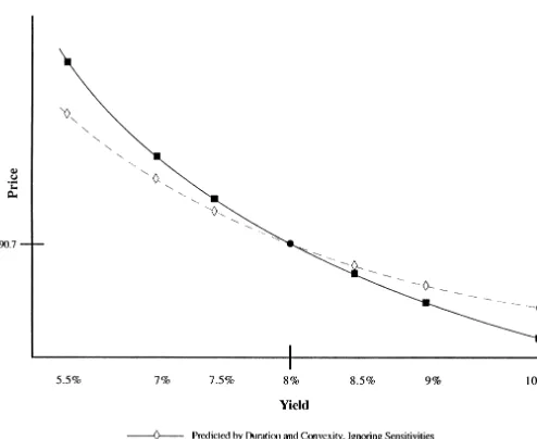
Figure 2. Price/yield relationship for different sensitivities.
put is deeply “out-of-the-money.” Therefore as credit risk asset values and interest rates to increase duration and a posi-tive relation to decrease duration, we expect a greater differ-increases (junior bonds) and more nodes become sensitive to
interest rate changes, there will be a greater impact on duration ence between the durations of the two issuer types the steeper the term structure.
and convexity. Thus the increased riskiness of junior debt should cause duration to be more heavily impacted by
interest-Convexity Hypotheses
rate sensitivity. Extensive empirical testing for a sensitivity
effect on bond returns has been performed in Appendix B. The impact of interest-rate sensitivity on convexity is more Regressions of bond returns on duration and a proxy for complex than for duration. As discussed previously a negative sensitivity (φ) show a strong significant impact. relation should amplify any price change due to rate changes Altering the initial term structure directly affects the future while a positive relation will lessen the change. This makes rates determined by the Kishimoto (Ho and Lee) model. In the impact upon duration easy to predict, but with convexity particular, increasing the upward slope causes future rates to we are concerned with the magnitude of the respective positive be higher. In our model we examine how the slope interacts and negative shift effects.
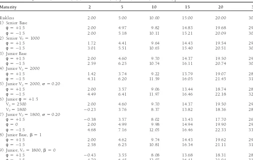
Table 1. Duration Calculations
Base Parameters:m 50.02,s 50.15, V0(senior)51500, V0(junior)52500,d 50.997, p50.5
Maturity 2 5 10 15 20 30
Riskless 2.00 5.00 10.00 15.00 20.00 30.00
1) Senior Base
φ5 11.5 2.00 4.97 9.82 14.83 19.68 29.52
φ5 21.5 2.00 5.18 10.11 15.21 20.09 30.45
2) Senior V051000
φ5 11.5 1.72 4.41 9.64 14.43 19.54 29.40
φ5 21.5 3.01 5.51 10.65 15.40 20.51 30.40
3) Junior Base
φ5 11.5 2.00 4.60 9.70 14.37 19.50 29.28
φ5 21.5 2.59 6.25 10.74 16.11 20.74 30.72
4) Junior V052000
φ5 11.5 1.42 3.74 9.22 13.79 19.07 28.85
φ5 21.5 4.31 6.20 11.59 16.05 21.45 31.43
5) Junior V052000,s 50.20
φ5 11.5 2.00 3.57 9.06 13.44 18.74 28.19
φ5 21.5 4.49 6.41 11.97 16.46 22.18 32.92
6) Juniorφ5 11.5
V052500 2.00 4.60 9.70 14.37 19.50 29.28
V051800 20.23 3.76 8.37 13.82 18.36 28.14
7) Junior V051800,s 50.20
φ5 11.5 20.38 3.57 8.02 13.43 17.70 26.86
φ50 2.00 4.99 9.98 14.94 19.90 29.80
φ5 21.5 4.68 7.16 12.05 16.46 22.33 33.37
8) Junior Base,b 51
φ5 11.5 2.00 4.62 9.74 14.43 19.62 29.54
φ5 21.5 2.58 6.25 10.81 16.34 21.11 31.66
9) Junior, V051800,b 50
φ5 11.5 20.43 3.55 8.08 13.68 18.31 28.54
φ5 21.5 4.70 6.45 12.07 16.41 21.94 31.94
impact on this relationship when the issuing firm’s asset value value to reduce both duration and convexity and a negative relation to increase both duration and convexity.
is impacted by interest rates.
Consider three distinct issuers, each with a different rela- The assumption of equal default risk is necessary to have the bond values of all three sensitivities begin at the same tion to interest rates: one with φ equal to zero, one with
sensitivity less than zero, and the last one greater than zero. point on the graph in Figure 2. To prove that the curvature changes we must verify that all three converge at the “end” Assuming all three firms have equal, nonzero default risk, an
interest rate of zero will cause the debt of each to be of equal of the graph, where yields become extremely large. Zero value is only achieved asymptotically when the interest rate becomes value (something less than face value due to the positive
probability of default). However, as the interest rate increases infinite. Therefore all three lines will converge to zero and will have imperceptibly different values at extremely high each issue will be affected differently. The bond withφ5 0
(no asset value sensitivity) represents the standard price/yield rates. If all three begin at the same point, have different slopes (durations), but the same values at the “end,” they must have tradeoff and its curve will lie between the other two. Ifφ.
0, asset value rises with interest rates. This should increase different curvatures (convexities).
The slope of the initial term structure should impact the the value of the debt relative to that of the insensitive firm’s
debt. The tradeoff will still be convex but flatter than with degree to which convexity is affected by the relation between asset value and interest rates. The Ho and Lee (1986) process
φ50. Therefore the convexity of this bond should be lower
than that for an issuer unrelated to interest rate changes. used in the Kishimoto (1989) model bases the size of future interest rate movements on the spread of rates in the initial For firm assets negatively related to rates, the increasing
rate has a greater effect on bond value. The bond is discounted term structure. A more steeply sloped term structure will lead to larger movements in rates. Thus a steeper initial term at higher rates and the asset value is reduced by the higher
rates. Therefore its price/yield curve falls faster than the other structure will result in a larger spread of terminal period rates computed by the model. This larger spread should cause the two as rates increase (higher duration) and is more convex
Table 2. Difference between Junior and Senior Duration (Using
S(T)5 a 1 b
1
ln(T) 1002
Base Values)Maturity
where S(T) is the spot rate for T periods,aandbare
parame-s50.10,φ5 21.5 20 30
ters set at 0.05 and 1.5, respectively, in the base case and adjusted as described. b represents the slope of the initial A
term structure and ranges from20.5 to11, whilearanges Varysonly
from Table 1 from 0.03 to 0.08. A b of 1.0 results in a spread of 3.4% Senior 20.22 30.35 between 1-year and 30-year spot rates. (This spread was 4.7% Junior 20.61 30.71 in September 1992 for zero coupon U.S. Treasury strips.) s 50.20,φ5 21.5
The use of the equation allows easy adjustments of the term
Senior 20.61 30.81
structure and keeps the shape relatively simple.
Junior 21.30 31.85
s 50.22,φ5 21.5
Senior 20.63 30.85
Duration Results
Junior 21.47 32.31
The size of the sensitivity effect is dependent upon the riskiness s 50.25,φ5 21.5
Senior 20.65 30.90 of the debt, the steepness of the term structure, and the Junior 21.80 33.76 magnitude of the sensitivity parameter. Table 1 summarizes B
the results for duration calculations where five of the seven Varysand Change
cases address junior debt. Case 1 demonstrates the difference Leverage from
in durations for senior debt with base case parameters and Table 1
V0(senior)51000 and V0(junior)52000 sensitivities of11.5 and 21.5. It shows that the debt with
Senior 20.53 30.61 sensitivity of21.5 has greater duration for maturities greater
Junior 21.05 31.06
than two but the difference is less than one year at a maturity s 50.20,φ5 21.5
of 30. Case 2 shows the effect of increasing the riskiness of
Senior 20.84 31.05
Junior 22.43 33.46 the debt by lowering the asset value for the senior debt issuer s 50.22,φ5 21.5 to $1,000. Note that the firm still has some equity as the Senior 20.88 31.11 present value of debt is less than face value. Here the difference
Junior 22.86 34.87
between sensitivities illustrates the impact of increased riski-s 50.25,φ5 21.5
ness. The difference in durations is one full year or more for
Senior 20.93 31.20
Junior 23.83 43.11 almost all maturities which is a large proportionate difference for shorter maturities. For example, at a maturity of two years the duration withφ5 21.5 is 75% greater than forφ5 11.5 (3.01 versus 1.72). Importantly, duration exceeds maturity for used in the model. Therefore a steeper slope should magnify negative φ cases but not when φ is positive in all Case 2 the difference between convexities of negatively and positively examples.
sensitive assets. As with duration we should see a greater effect In general junior debt displays a greater response to changes for riskier junior debt in all cases. in parameters. Case 3 shows a greater difference than that occurring for senior debt. With the base case parameters, junior debt has a duration difference of about 1.5 years
be-Results
tween sensitivities of 11.5 and 21.5 for maturities of 15 years or more. The proportional difference for short maturities For our simulations we use the following base case variablesfor senior debt: firm-specific asset growth (m) of 2%, standard (under 10 years) is quite large. Case 4 shows that as initial asset value is decreased to $2,000 the difference in duration deviation of growth (s) of 15%, sensitivity (φ) of 0, initial
asset value of $1,500, and face value of debt of $1,000. For is very close to 2.5 years even at very short maturities. At a maturity of 2 years the duration of the negative sensitivity is junior debt the only changes are that beginning asset value
is raised to $2,500 and the face value of both junior and more than double that of positive sensitivity. When the stan-dard deviation is increased to 0.20 (Case 5) the duration senior debt is $1,000. The leverage is similar to that used by
Cakici and Chatterjee (1993) in their analysis of bank debt. spread increases slightly with maturity, reaching more than 4 full years at a maturity of 30 and is 2 or more across all Of course, many banks are even more leveraged, and the
leverage used is similar to that of many nonfinancial firms maturities. Note that duration substantially exceeds maturity (for example, 4.49 versus a maturity of 2) when a negative with large issues of high yield (junk) bonds. See Cakici and
Chatterjee (1993, footnote 5) for examples of high leverages. sensitivity is used in Vases 3, 4, and 5.
We find that asset value (leverage) and volatility (s), param-The initial term structure used in our simulations is created
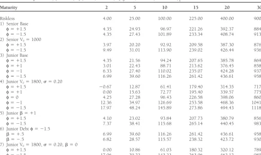
Table 3. Convexity Calculations
Base Parameters:m 50.02,φ50.15, V0(senior)51500, V0(junior)52500,d 50.997,p50.5
Maturity 2 5 10 15 20 30
Riskless 4.00 25.00 100.00 225.00 400.00 900.00
1) Senior Base
φ5 11.5 4.35 24.93 96.97 221.26 392.37 884.41
φ5 21.5 4.35 27.43 101.89 233.34 408.74 913.26
2) Senior V051000
φ5 11.5 3.97 20.20 92.92 209.58 387.30 876.86
φ5 21.5 9.49 31.01 113.90 239.02 426.44 936.92
3) Junior Base
φ5 11.5 4.35 21.56 94.24 207.65 385.78 869.05
φ5 11 3.01 22.43 88.71 213.62 376.45 858.34
φ5 21 6.33 27.40 110.02 235.07 424.28 937.08
φ5 21.5 6.99 39.60 116.26 261.42 436.61 958.25
4) Junior V051800,s 50.20
φ5 11.5 20.67 12.87 61.41 179.40 314.35 717.78
φ5 11 0.00 15.63 72.77 195.40 339.57 775.91
φ50 4.25 27.28 96.43 226.58 398.06 860.85
φ5 21 12.36 34.97 126.69 253.58 468.36 1041.03
φ5 21.5 17.97 48.24 145.89 273.86 494.43 1118.60
5) Juniorb 5 11
φ5 11.5 4.10 23.02 93.84 207.73 380.79 856.51
φ5 21.5 7.37 38.41 115.68 265.14 440.45 983.79
6) Junior Debtφ5 21.5
b 5 1.5 6.99 39.60 116.26 261.42 436.61 958.25
b 5 2.5 6.82 28.57 115.57 238.32 423.72 930.06
7) Junior V051800,s 50.20,b 50
φ5 11.5 0.00 10.86 61.03 180.32 320.12 789.23
φ5 21.5 17.06 39.22 143.22 263.06 462.12 985.50
cases. Case 6 shows the duration for two issues with sensitivity where the only difference is Case 8 assumes a greater term structure slope (than Case 3) and Case 9 assumes a lesser parameters of11.5 each but where one has an asset value of
$1,800 and the other $2,500. Note that the difference between slope (than Case 7). The spread between 30-year durations is greater in Case 8 (than Case 3) but less in Case 9 (than the two is typically just over 1 year past a maturity of 5 years.
Also note that a negative value for duration is present at the Case 7).
The difference between senior and junior duration is quite 2-year maturity. This occurs because the reduction in default
risk from the increased asset value dominates the effect of sensitive tosand leverage (initial asset value). Table 2, panel A, contains duration assvaries for long maturities ifφis21.5 higher discount rates on the bond price.
The most striking results are achieved when the junior where greater volatility increases the difference and junior duration always exceeds senior. All other parameters are un-debt is used with asset value of $1,800 and standard deviation
of growth of 0.20 [parameters which are consistent with those changed from Table 1. For example, ifsis 0.10, the difference in duration for a 30-year maturity is only 0.36 (30.71 versus used by Cakici and Chatterjee (1993)]. Case 7 illustrates this
result where the difference in duration between sensitivities 30.35) but 2.86 (33.76 versus 30.90) forsof 0.25. Table 2, panel B, contains variation insand also lowers asset values of11.5 and21.5 is never less than three periods and grows
to over six at a maturity of 30. At shorter maturities the (greater leverage) so that the difference in duration grows even more dramatically assincreases. That is, the difference negatively related duration can be more than double the
posi-in duration is almost 12 when maturity is 30 andsis 0.25. tively related.
Examination of the table reveals that the increase in duration Case 7 also displays the results of zero sensitivity. Note
difference is due to junior duration being quite sensitive to that even with the low asset value and the high standard
swhile senior is not very sensitive. deviation (s 5 0.20) the durations are still very close to
that of the riskless shown at the top of the table. This again
Convexity Results
demonstrates the importance of the sensitivity,φ, relative to
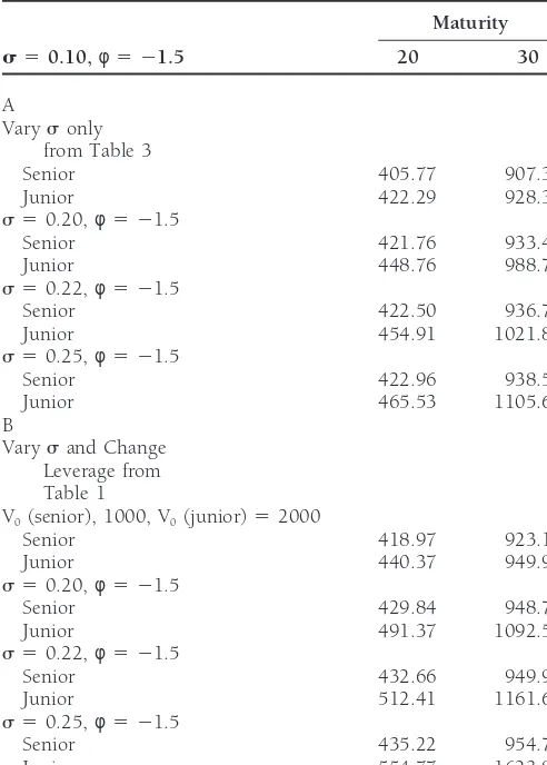
Table 4. Difference between Junior and Senior Convexity (Using debt. Case 5 usesb 5 11 instead of10.5 and shows the base values) convexity differences resulting from the increased slope of the
initial term structure. Note that with the steeper slope the
dif-Maturity
ference due to the sensitivities is greater. The difference in
s50.10,φ5 21.5 20 30
convexities grows from about 90 for Case 3 to almost 130 in Case 5, at a maturity of 30 years. However, the direction of A
Varysonly this term structure slope is not as important as the magnitude. from Table 3 Case 6 compares convexities of negative sensitivity issues un-Senior 405.77 907.34 der both an upward (b 50.5) and a downward sloping term
Junior 422.29 928.37
structure (b 5 20.5). The two convexities are similar because s 50.20,φ5 21.5
each slope creates similar differences between spot rates for
Senior 421.76 933.49
Junior 448.76 988.75 1 and 30 years which will make the spread of terminal rates s 50.22,φ5 21.5 projected by the Kishimoto (1989) model approximately the Senior 422.50 936.70 same under each slope. Thus, while the different slopes may
Junior 454.91 1021.89
affect the relative value of the debt, it has less impact on the s 50.25,φ5 21.5
debt’s sensitivity to rate changes.
Senior 422.96 938.55
Junior 465.53 1105.65 Case 7 in Table 3 shows the impact of a flat term structure B (b 50). The flat term structure creates a set of convexities Varysand Change
that have considerably less variation in value for long maturi-Leverage from
ties than in Case 4 because a flat term structure implies no Table 1
change in expected interest rates. This term structure shape V0(senior), 1000, V0(junior)52000
Senior 418.97 923.12 does not result in convexities exactly equal to the riskless case Junior 440.37 949.91 due to nonzero asset value volatility.
s 50.20,φ5 21.5
Similar to Table 2, the difference between junior and senior
Senior 429.84 948.77
convexity is quite sensitive tosand leverage. Table 4, panel
Junior 491.37 1092.57
s 50.22,φ5 21.5 A, shows convexity as s varies for long maturities if φ is Senior 432.66 949.93 21.5 where greater volatility increases the difference quite Junior 512.41 1161.62 dramatically and junior convexity always exceeds senior. All s 50.25,φ5 21.5
other parameters are the same as in Table 3. For example, if
Senior 435.22 954.77
sis 0.10, the difference in convexity for a 30-year maturity
Junior 554.77 1623.85
is only 21.03 (928.37 versus 907.34) but 167.10 (1105.65 versus 938.55) ifsis 0.25. Table 4, panel B, again varies s but at a lower asset value so that the difference in convexity positive. Case 1 shows the senior base case convexities with
grows even more dramatically withs. That is, the difference sensitivities of11.5 and21.5. Notice that each convexity is
in convexity is 669 whensis 0.25 and maturity is 30. Exami-quite close to that of a riskless bond shown at the top of the
nation of the table for a 30-year maturity reveals that the table. Case 2 reveals that as initial value is decreased to $1,000
increase in convexity difference is due to junior convexity the difference between sensitivities grows significantly and
being quite sensitive while senior is not very sensitive. increases with maturity. At a maturity of two, the convexity
of the negativeφis more than twice the positive.
Junior debt shows much greater difference in convexities
Conclusion
and is again much more sensitive to parameter changes thanThis article has demonstrated some of the important effects senior. Case 3 shows the base case positions with sensitivities
that relating asset value to interest rates can have on a firm’s of11.5, 11,21, and 21.5 where, again, convexity
differ-debt. We have incorporated a non-flat term structure and ences increase with maturity. Changing the initial asset value
volatile interest rates, and then related these to the assets of provides significant changes to the convexity of junior debt.
the firm. The results indicate that if asset value is negatively Case 4 shows that when initial asset value is reduced to $1,800
related to interest rates, debt will be more sensitive to changes and the standard deviation is raised to 0.20 the difference
in rates than an issue with a positive or no relation. The junior between convexities becomes very large—over 400 between
debt durations and convexities for risky debt can be much the high and low sensitivities at 30-year maturities. Notice
different than those of riskless debt and senior debt where that when the sensitivity is equal to zero, convexity is much
this difference becomes more pronounced when interest-rate closer to that of the riskless bond. This again verifies the
sensitivity is included. No previous research has analyzed the importance of the relation between asset value and interest
convexity of default risky bonds. With a negative relation we rates.
Ilmanen, Antti, McGuire, Donald, and Warga, Arthur: The Value of riskless levels, and duration can exceed maturity. When a
Duration as a Risk Measure for Corporate Debt.Journal of Fixed
positive relation exists duration and convexity are reduced
Income4 (March 1994): 70–76. from those of riskless debt. Additionally, the results displayed
Kahn, Ronald N., and Lochoff, Roland: Convexity and Exceptional by junior debt are more dramatic than those of senior debt.
Returns.The Journal of Portfolio Management16 (Winter 1990): This inherent riskiness of junior debt seems to magnify the 43–47.
impact of the asset’s sensitivity to interest rates. Greater lever- Kishimoto, Naoki: Pricing Contingent Claims under Interest Rate age and volatility magnify the difference between junior and and Asset Price Risk.Journal of Finance44 (July 1989): 571–589. senior duration and convexity. The shape of the term structure Longstaff, Francis A., and Schwartz, Eduardo S.: A Simple Approach can play a critical role in determining duration and convexity. to Valuing Risky Fixed and Floating Rate Debt.Journal of Finance
50 (July 1995): 789–819. Thus duration defined as the sensitivity of bond price is
clearly inconsistent with duration defined as the weighted Merton, Robert C.: On the Pricing of Corporate Debt: The Risk Structure of Interest Rates. Journal of Finance 29 (May 1974): average timing of cash flows. As the risk of the issue increases,
449–470. these effects are dramatically enhanced. Although this is
obvi-Nawalkha, Sanjay: A Contingent Claims Analyses of Interest Rate ously important for financial institutions, many other firms
Characteristics of Corporate Liabilities. Journal of Banking and
are affected by interest rates in some way making many of
Finance20 (2 1996): 227–245. the issues discussed in this article important for any bond
Prisman, Eliezer, and Shores, Marilyn: Duration Measures for Specific investor. A bond portfolio manager using simple Macaulay
Term Structure Estimation and Applications to Bond Portfolio duration computed from a weighted average of cash flows Immunization. Journal of Banking and Finance12 (Sept. 1988): may well have an inaccurate measure of price volatility. 493–503.
Rendelman, Richard J., Jr., and Bartter, Brit J.: Two State Option The authors thank Ajay Madwesh for his exceptional work in programming Pricing.Journal of Finance34 (Dec. 1979): 1093–1110. the model used in this article. Also, we thank Louis Ederington for helpful
Rendleman, Richard J., Jr., and Bartter, Brit J.: The Pricing of Options comments.
on Debt Securities.Journal of Financial and Quantitative Analysis
15 (March 1980): 11–24.
Schnabel, Jacques A.: Is Benter Better? A Cautionary Note on
Max-References
imizing Convexity.Financial Analysts Journal46 (Jan./Feb. 1990): Bierwag, G. O.: Immunization, Duration, and the Term Structure of 78–79.
Interest Rates.Journal of Financial and Quantitative Analysis 12
Stock, Duane, and Simonson, Don: Tax Adjusted Duration for Amor-(December 1977): 725–742.
tizing Debt Instruments.Journal of Financial and Quantitative
Anal-Black, Fischer, and Cox, John: Valuing Corporate Securities: Some ysis23 (Sept. 1988): 313–327. Effects of Bond Indenture Provisions.Journal of Finance31 (1976):
361–376.
Cakici, Nusret, and Chatterjee, Sris: Market Discipline, Bank Subordi-
Appendix A
nated Debt, and Interest Rate Uncertainty.Journal of Banking andFinance32 (Aug. 1993): 747–762. The excess returns to a bond are functions of the perturbation terms h(1) and h*(1). Given that we model varying degrees Chambers, Don, Carleton, W. T., and McEnally, R. W.: Immunizing
Default Free Bond Portfolios with a Duration Vector.Journal of of sensitivity (φ) of asset value to interest rates, the excess Financial and Quantitative Analysis23 (March 1988): 89–104. returns become fairly complex functions of h(1) and h*(1) as
Chance, Don M.: Default Risk and the Duration of Zero Coupon shown below.
Bonds.Journal of Finance45 (March 1990): 265–274. In our model, asset value and interest rate movements are DeAlessi, Louis: Do Business Firms Gain from Inflation?Journal of related in the following manner
Business48 (April 1964): 162–166.
gnj5 eφ(Rnj(1)) but Rnj(1)5 2lnDnj(1).
Fisher, Lawrence, and Weil, Roman L.: Coping with the Risk of Interest-Rate Fluctuations: Returns to Bondholders from Naive
Thusgnj5 eφ(2lnDnj(1)) 5 Dnj(1)2φ.
and Optimal Strategies.Journal of Business20 (Oct. 1971): 408– 431.
Looking at the first subperiod of the first period Garman, Mark B.: The Duration of Option Portfolios. Journal of
Financial Economics14 (June 1985): 309–316. g115 D11(1)2φ 5 g
up, and g105D10(1)2φ5 gdown.
Grantier, Bruce J.: Convexity and Bond Performance: The Benter,
Here, the Better.Financial Analysts Journal44 (Nov./Dec. 1988): 79–82.
Ho, Thomas S. Y.: Managing Illiquid Bonds and the Linear Path
D11(1)2φ 5
1
Space.Journal of Fixed Income2 (March 1992): 80–93.Ho, Thomas S. Y., and Lee, Sang-Bin: Term Structure Movements and Pricing Interest Rate Contingent Claims.Journal of Finance
D10(1)2φ 5
1
Hull, John:Options, Futures and Other Derivative Securities,
Table A1.
1
DPi,t1ci/12Pi,t
2
2rt5 b01 b1Di,t(2Drt)1 b2(φi)1 b3(SPDi,t22)1 ei,t
Adjusted Number of
b0 b1 b2 b3 R2 Observations
Aaa and 0.00077 0.8588 20.000309 0.0900 0.7954 1,371 Aa (2.288)* (69.11) (24.112) (7.271)
A-Ba 0.0024 0.7201 20.00014 0.1624 0.4143 8,299
(10.527) (60.149) (22.456) (17.958)
Aaa-Ba 0.0020 0.6345 20.000201 0.2077 0.3934 9,670 (7.899) (44.273) (23.228) (21.004)
*t-statistics in parentheses
change in asset value due to interest rate changes from one EQRETi,t5 a0 1 a1Drt.
period to the next. Within gup and gdown, both Doo(2) and
The regression coefficient a1 is then used to represent
Doo(1) are given by the initial term structure used to price the
sensitivity (φ) to interest rate changes. Stock returns are from risk-free bond. Thus the only arbitrage possibility results from
the Center for Research in Security Prices (CRSP) where stock the perturbation functions h(1)2φ and h*(1)2φgiving the no
price behavior is used as a proxy for asset value. The above arbitrage requirement that
equation is estimated over a minimum of four years depending ph(1)2φ1(12p)h*(1)2φ51 on availability of continuous stock and bond prices from
January 1985 to December 1993. Firms without continuous Exhaustive simulations testing that this requirement holds
prices were eliminated. The specification as used in IMW is have been performed. The simulations assume realistic values
for d, φ values within the range used in this research, and
1
DPi,t1ci/12Pi,t
2
2rt5 b01 b1Di,t(2Drt)1 b2(φi)
varyingpvalues. Realisticdvalues are those that yield realistic interest volatilities using Hull’s (1989) formula for per annum
1 b3(SPDi,t22)1 ei,t
interest rate volatility.ds less than 0.995 are thus very unusual because smallerds give volatilities over 50% which are unreal- DP
i,tis bond price change for bond “i” from month “t-1” to
istically high.φvalues of close to zero andd values close to “t,” P
i,tis price in month “t,” and ciis the annual coupon. Di,t
one give a resultph(1)2φplus (12 p)h*(1)2φequals 1 with
is the duration of the bond,Drtis the change in the one year
accuracy beyond the 8th decimal place (e.g., 1.00000006). If Treasury bill rate, andφ
i is the sensitivity of stock price to
φis, say, 1.5,d 50.995, andp 50.5, the result is accuracy changes in interest rates,a
1from above. SPD is a default risk
to the sixth decimal place (e.g., 1.000002). variable used by IMW and is calculated as return on the bond less the risk free rate for time t-2. IMW use a lag to eliminate potential bias because there will be no contemporary prices
Appendix B
on the left and right sides of the regression. (IMW find
convex-Sensitivity of Asset Value to Interest Rate
ity does not add much explanatory power and we foundChanges and the Impact on Bond Returns
similar results.) The database of bond prices and returns used was the Fixed Income Data Base (University of Wisconsin at Our model suggests that a bond’s sensitivity to interest rateMilwaukee). Due to an expectation of greater interest-rate changes can be significantly affected by the relation to interest
sensitivity, only bonds from financial firms were used. The rates. If assets are negatively (positively) related to interest
time period used was the same as that used to estimate the rates, its debt will be more (less) sensitive to interest rate
sensitivity in the EQRET regression. Thus 71 firms were used changes. To provide empirical testing of such an hypothesis,
where some firms had more than one issue included. Callable we follow Ilmanen, McGuire, and Warga (1994) (IMW), who
and convertible bonds were excluded. As in IMW, bonds of examined the ability of duration to measure interest-rate risk
less than one year maturity were not included because dura-in corporate debt. Their basic procedure was to regress excess
tion for such short-term bonds is greatly affected by the pass-returns upon duration, convexity, and default risk. They
con-ing of one month. Our model predicts a negative relation clude that duration explains a large proportion of returns
between excess returns andφsuch thatb2 is expected to be
although the proportion declines as credit rating declines.
negative. To test whether asset sensitivity to interest rate changes
Table A1 contains the results where regressions for both affects bond returns, we add an explanatory variable which
high grade (Aaa and Aa) and lower grades (A, Baa, Ba) are is the result of regressing monthly equity (stock) returns
(EQ-given. Like the IMW results, the R2 value is lower for lesser
RET) for firm i upon changes in the one-year U.S. Treasury
grades of bonds were estimated. Small sample size discourages In this formulation, the parameterφis measured with error. This error could potentially bias the estimate of the standard regressions for each rating class. As hypothesized, the
sensitiv-ity measure is significantly and negatively related to excess errors in the second regression. To address this potential, simulations were run based on the standard error of estimate returns for both sets of bonds. Thus, bond returns are in fact
sensitive to asset values. Also, the return attributed to this of a1 in the first regression equation. In all, 300 different
values ofφfor each firm were used with the values randomly sensitivity can be a large proportion of total excess return.
For example, the average monthly excess return is 0.0033 for selected from a normal distribution with mean equal to the least squares estimate ofa1in the first regression and standard
Aaa and Aa bonds and the minimum φ value is 210.747.
Thus, 210.747 times the coefficient 20.000309 is 0.0033 deviation equal to the standard error ofa1. The residual errors
for the simulations were averaged across all 300 regressions which is 100% of the average return. If the average φ of
23.664 is used, the result is 23.664 times 20.000309 or and compared to those from the second regression. The pro-cess was repeated three times and in no case were the values 0.0012 which is more than one-third the average monthly