*Corresponding author. Tel.: 5105; fax: 1-405-744-5180.
E-mail address:[email protected] (H.S. Lau)
Demand uncertainty and returns policies for a seasonal
product: An alternative model
Amy Hing-Ling Lau, Hon-Shiang Lau*, Keith D. Willett
College of Business Administration, Oklahoma State University, 201 Stillwater, OK 74078-055, USA
Received 4 August 1998; accepted 25 May 1999
Abstract
Marvel and Peck [International Economic Review 36 (1995) 691}714] considered the following seasonal-product problem: A manufacturer sets wholesale price ($p
8/unit) and return credit ($r/unit); the retailer then sets retailer price
($p
R/unit) and order quantity (Q). How should the manufacturer setp8 andr? Demand uncertainty consists of two
components:`valuationaand`customers'arrivalsa. Our more realistic models reveal e!ects unobservable from
Mar-vel}Peck's. E.g.: (i) Setting r'0 bene"ts the manufacturer much more than the retailer. (ii) `Valuationa (but not
`customer-arrivala) uncertainty is imperative for the retailer; without it, the manufacturer can setp
8andrsuch that he
reaps most of the pro"ts. ( 2000 Elsevier Science B.V. All rights reserved.
Keywords: Newsboy problem; Pricing; Returns policy; Demand uncertainty; Supply-chain interaction
1. Introduction
Recently, Marvel and Peck [1] posed the follow-ing problem in the economics literature:
The manufacturer wholesales a product to the retailer for $p
8/unit. Units of the product that the retailer could not sell may be returned to the
manufacturer for a $r/unit reimbursement. The
retailer buysQunits from the manufacturer and attempts to retail them to his customers at $p
R/unit. For any given p8 and r set by the
manufacturer, the retailer will setp
R andQthat
maximize the retailer's own expected pro"t. Re-cognizing this, how would (or should) the manu-facturer setp
8 andr?
The model used by Marvel and Peck [1] to answer the above questions uses a couple of key assumptions. There are several di!erent plausible variations of these assumptions; unfortunately, us-ing a di!erent variation leads to very di!erent model behavior (i.e., conclusions on how the manu-facturer and retailer would/should set their prices and quantities). The purposes of this paper are to: (i) present some realistic variations of the Mar-vel}Peck (hereafter `MPa) model; (ii) sketch the necessary solution methodologies for these vari-ations; and (iii) use the numerical solutions
ob-tained from the modi"ed models to present
alternative answers to the question posed by MP. It will be seen that the answers obtained with our
models di!er considerably from the answers
ob-tained from MP's model. This paper assumes fam-iliarity with MP's [1] paper, and uses as much as possible the same symbols de"ned there; also, their 0925-5273/00/$ - see front matter (2000 Elsevier Science B.V. All rights reserved.
background discussion of the problem will not be repeated.
1.1. Basic dexnitions
The`manufactureraincurs a manufacturing cost of$c/unit for a product, he wholesales them to the `retaileraat $p
8/unit, and pays the retailer$r/unit for returned (unsold) units. The retailer buys
Q units from the manufacturer and retails to his
`customersaat$p
R/unit.`Qamay be subscripted as
`QRa,`QMaor`QIawhen it is desirable to specify the party (retailer, manufacturer, or the vertically integrated"rm) making the Q-decision. Similarly, nM,nRandnI denote the expected pro"t of, respec-tively, the manufacturer, the retailer and the integrated"rm.
Random variables will be denoted by bold letters. In MP [1] the random demand is character-ized by two independent random components:
(i) v: the valuation or `reservation pricea retail customers place on the product; with density f()), distribution function F()), and support
[v,v6]. A customer will only purchase the prod-uct if the customer's actual v-value equals or exceeds the retail pricep
R.
(ii) m: the number of customers who arrive during a particular market cycle; with density g()),
distribution functionG()), and support [m,m6 ].
MP further assumed that each of the m
cus-tomers who arrives will purchase (exactly)oneunit ifv*p
R, and zero otherwise. MP considered three
cases:
Case 1: mdeterministic butvstochastic.
Case 2:vdeterministic butmstochastic.
Case 3:bothvandmare stochastic.
In addition to the above symbols de"ned in MP [1], we de"ne
di demand from a single customeri
D the total demand from the m customers,
with support (D,DM); h()) and H()) are D's
density and distribution function, respec-tively
nCr n!/[r!(n!r)!]
P
"(pR) [1!F(pR)], the probability that a
cus-tomer will buy at retail pricep
R
P
/ 1!P"
For a standard normally distributed variable z&N(0, 1), its density and distribution function are denoted by, respectively,u(') andU(').
For any random variable x, let k
x"E(x), kk(x)"E(x!k
x)k "kth central moment of x,
andp
x"Jk2(x).
The optimal value of a decision variable x is
denotedxH. The optimum of an objective variable (say)noptimized over one decision variable is de-notednH; whereasnHHis the value optimized over two decision variables.
1.2. Brief literature review
The seasonal product MP considered is closely
related to the `newsboy problemain the MS/OR
literature. The problem is brie#y de"ned below:
The stochastic demand D of a single-period
product (e.g., a newspaper) is represented by a given probability distribution. The`unit costato the retailer is"xed. The problem is to determine order quantityQ(and perhaps retail pricep
R).
Compared to the preceding structure, MP's
problem has (among others) two important addi-tional features:
(i) While the newsboy problem (as in most
MS/OR inventory models) characterizes de-mand uncertainty by a statistical dede-mand dis-tribution, MP's model perceives two separate
components a!ecting demand uncertainty:
vandm. Both MP's and our studies show that these two uncertainty components a!ect opti-mal decisions quite di!erently.
(ii) Practically all papers in the huge MS/OR `newsboya literature (see references in, e.g., Khouja [2] and Lau [3]) consider only how an integrated `manufacturer}retailer entitya would deal with the retail market; or, equiva-lently, they assume thatp
8andrare"xed and hence the manufacturer has no decision vari-able. MP's model considers the interaction
1The original Pasternack's [4] relationship (i.e., his Eq. (10)) is more general, i.e., it contains several additional factors which are not needed in our current problem, hence they have been` sim-pli"ed outain our Eq. (2).
are now recognized as two separate entities. This adds two more decision variables (p
8and r) to the problem.
Pasternack [4] is the"rst to consider manufac-turer/retailer interaction in the newsboy context. He assumed that the retail price pis"xed by the market, but the retailer is entitled to return to the manufacturer all unsold units for a refund of $r/unit. De"ning`channel e$ciencyaas
E
&"(nHHM #pHHR )/nHI. (1)
Pasternack showed that: (i) a manufacturer's deci-sion ofr"0 will lead to`E
&(1a; (ii) the manufac-turer can enforce `E
&"1a by setting a ` channel-coordinatinga(w,r) (withr'0) such that the fol-lowing relationship is satis"ed:1
(p
R!c)(pR!r)"(pR!w)pR. (2)
He also pointed out that: (i) there exists in"nite sets of (w,r)-values that satisfy (2); and (ii) di!erent channel-coordinating (w,r)s lead to di!erent ways of splitting HHV between the manufacturer and the retailer. However, Pasternack [4] did not address the mechanism for regulating this pro"t split be-tween the manufacturer and the retailer (or, in other words, how does or should the manufacturer pick one implementable pair of (w,r)-values out of the in"nite possibilities). Essentially, MP not only attempted to answer the above question, but they also did so for an extended model whose stochastic
demand is decomposed intovandm.
Pricing between manufacturers and retailers has been studied by many (see, e.g., [5,6] and their references), but mostly in the context of non-sea-sonal products with deterministic (though possibly price-dependent) demands. Recently Padmanab-han and Png [7] also considered manufac-turer/retailer interactions in a seasonal product
with uncertain demand. Two fundamental di!
er-ences between Padmanabhan}Png's and the
news-boy}MP models are: (i) Padmanabhan}Png's
model assumes that the demand uncertainty is re-solved before the retailer setsp(and hence before
the selling begins), whereas the newsboy}MP
models assume that demand uncertainty exists throughout the selling season; (ii) market uncer-tainty is represented by a (discrete) Bernoulli distri-bution in Padmanabhan}Png's model, but by more
comprehensive formats in the newsboy}MP
mod-els. Similar di!erences apply between the news-boy}MP models and the other models cited in [7].
1.3. Overview
Section 2 shows that, under the stochastic-vCase 1, how a di!erent interpretation of v will lead to very di!erent formulations and solutions. Section
3 shows that, under the stochastic-mCase 2, how
a di!erent assumption on the manufacturer} re-tailer relationship will also lead to very di!erent formulations and solutions. Section 4 gives a sum-mary and brie#y discusses fruitful extensions.
2. The assumption on whether di4erent customers have di4erent v
There are at least two alternatives in interpreting the statement of`P
"(pR)"[1!F(pR)]ade"ned in
Section 1.1:
Alternative A: At the end of the market period the
single realized value ofvbecomes known, and (as stated in [1, p. 699]) `all buyers have the same reservation priceva.F()) governs the realization of
this universalv-value.
Alternative B: Di!erent customers have di!erent
actualv-values*whose distribution followsF()).
The probability that any given customer will buy is P""[1!F(pR)]. Given any P" (assume
0(P
"(1), some customers (roughly 100P" per-cent of them) will end up buying, others will not.
To illustrate clearly the di!erence between the two alternatives, assume that: (i) there arem"1000 customers; (ii)v&;(0, 1) (i.e.,F(v)"v, like the one used in MP's numerical illustration); and (iii)p
R"
0.8 (pre-set). Under Alternative 1, Prob(v(p
R)"
assumed deterministic, there is no way forDto be anything but either 0 or 1000. Under Alternative B, P
""0.2, hence the actualDobserved at the end of the period can have any value between 0 and 1000, the probability of observingMD"runitsNis given by the binomial probability [
1000Cr](0.2)r(0.8)1000~r. For example, in a CD/records store, if Alternative A applies, the observed demand for each of the many titles carried would be either 0 or a very high value (equal to the number of potential buyers of the title that visited the store). If Alternative B ap-plies, the observed demands of di!erent titles would
be a more continuous range of values. MP's [1]
model uses Alternative A.
It appears that Alternative B is at least as plaus-ible as Alternative A. This section shows that sub-stituting Alternative B into MP's model leads to very di!erent mathematical formulations and re-sults for Case 1 (where only v is stochastic); also, many of these results appear to be at least as plausible as the Alternative A results.
2.1. Using Alternative A in Case 1(no arrival
uncertainty)
A convenient consequence of using Alternative A is that, as MP [1, p. 694] stated:`ifmis known, the (deterministic-m) problem can be reduced to that of dealing with a representative (customer)a. Since the retailer's problem is to maximize his own expected pro"tnR, considering only one represen-tative customer gives (as stated in the expression above MP's equation [1, Eq. (2) p. 694])
nR1"max [p
R[1!F(pR)]#F(pR)r!p8, 0] (3a)
"max [(p
RP"#rP/!p8), 0] (3b) (using our new notationsP
"andP/). Thus, the de-cision is:`IfnR1'0, order; otherwise, do not or-dera. To illustrate, consider a simpli"ed situation
wherep
R andp8are already"xed. Assume m"1000, p
R"4, P""0.6, r"1, c"1. (4) Ifp
8"2.9, then substituting thisp8-value and the values in (4) into (1) gives
nR1"max [(4]0.6#1]0.4!2.9), 0]
"max [!0.1, 0]"0.
Hence,
whenp
8"2.9,QH"0 and Retailer's Aggregate Pro"t (nR1)"$0. (5a)
In contrast, if p
8"2.7, Eq. (1) becomes nR1"max [#0.1, 0]"0.1; hence,
whenp
8"2.7,
QH"1000 and nR"1000nR1"$100. (5b)
Simply put, the decision is:`QH"0 ifp
8*2.8; but QH"1000 units if p
8(2.8a. QH abruptly jumps
from 0 to 1000 whenp
8decreases from 2.8 to (say) 2.7999*this behavior comes from the logical and convenient consequence of ignoring the important factor m"1000 when one adopts Alternative A. The next subsection examines Alternative B: di! er-ent customers have di!erent realizedv-values.
2.2. Using Alternative B in Case 1(no arrival
uncertainty)
This study assumes thatmis su$ciently large so thatDunder Alternative B can be approximated by a normal distribution. This largemassumption is consistent with the current scenario of a manufac-turer using a retailer. If m is small (as when an industrial manufacturer sells to a few industrial users), it is more likely that a retailer is not used (it should, however, be emphasized that a smallm for-mulation requires only a straightforward extension f the following approach).
Under the Alternative B interpretation of F()),
the`demand per customeradi is a`Bernoulli dis-tributedarandom variable with k$"P
", and the mean and standard deviation of total demand Dare (see, e.g., [8])
k
D"mP""mk$, pD"JmP"P/. (6a) Substitutingm"1000 andP
""0.6 for the current case into (6a) gives
k
D"1000]0.6"600, p
D"J1000]0.6]0.4"15.492. (6b)
Also, whenmP
" andmP/ are both greater than 5,
D is very closely approximated by a continuous
if the retailer ordersQunits, the retailer's expected pro"t function is
n
whereQis a decision variable. Eq. (7) is the classical
`newsboy problema, and solving for`dnR/dQ"0a
gives
H(QH)"(p
R!p8)/(pR!r) or
QH"H~1[(p
R!p8)/(pR!r)]. (8)
H(QH) is commonly known as the `service levela
(hereafter`SLa), i.e., the likelihood thatnot all the merchandise (i.e., all the QHunits) are sold at the end of the season.
SinceH(z) is normal, we also have
H~1(y)"k
D#zp$,
wherez"U~1(y) (de"ned in Section 1.1). (9) Combining Eq. (4), (8) and (9) and using a standard normal table, we have
QH"600#15.49][U~1(0.3666)]"594.7
Combining Eq. (7) and (8) and simplifying, it can also be shown that, for any givenp
Randp8, when the retailer maximizes hisnR by orderingQH pre-scribed by Eq. (8), his resultant expected pro"t underanyh(') will be
and the results in [9] gives
nHR(p pected pro"t the retailer can extract from his mar-ket if he has perfect marmar-ket information (or if p
D"0), the second term amounts to the`expected value of perfect market informationa.
The following tabulation (obtained with Eqs. (4),
(8) and (11)) shows the `smootha variation of
QH and nHR(p
R) with p8 under Alternative B (the values of the other parameters are as given in (4)):
P prescribed by Alterative A, Eq. (5b) gavenR"100, which is considerably less than the corresponding nHR"761.72 given in (12) for Alternative B. Note also the drastically reduced but yet positivenHRwhen p
8moves from 2.50 to 3.95 under Alternative B. The above example (particularly the numerical approach) clari"es: (i) the di!erence between the MP'snR1-criterion (Eq. (3)) and our modi"ednR -criterion (Eq. (7)); and (ii) a basic characteristic of the current manufacturer}retailer problem that is unfortunately concealed by Eq. (3). nR (or nR1) of
Eq. (3) suggested that when p
8 exceeds $2.8, the retailer will setQ"0 because hisnR1is 0 (refer to (5a)); in other words, the model contains an internal
mechanism to enforce a relatively low p
8 (and hence a relatively high retailer's pro"t share).nRof Eq. (7) indicates that even when the manufacturer raisesp8to 3.95 (and beyond, as long as it is lower thanp
R"4), the retailer'snRwill still exceed 0 (see
mechanism to enforce a `reasonablea ratailer's pro"t share; instead, an additional`alternative op-portunityafactor is needed to enforce a relatively high retailer's share. A well-known analogy is the way pro"t is split between the landowners (aristo-crats) and the users (peasants) in many economies in the past and present. Similarly, urban street vendors (of, e.g., newspapers and imported or
`fancyaice-creams/soft-drinks) in many of today's
developing countries get a much smaller pro"t cut compared to either (i) the manufacturers/importers; or (ii) similar vendors in the developed countries. These vendors will get a larger pro"t share only when alternative employment opportunities force the manufacturers/importers to raise the retailers'
share in order to retain them. The next section (on Case 2) will consider the explicit imposition of a minimum required retailer's pro"t.
2.3. Solution of the no-arrival-uncertainty problem
with alternative B assumption
To clarify the implication of our Alternative B
interpretation of the statement `P
"(pR)"
[1!F(p
R)]a, the preceding subsections considered
situations with givenp
8 andpR. This restriction is
now removed for solving MP's Case 1 problem.
Whenp
Ras well asQR are the retailer's decision
variables, then by combining Eqs. (6a) and (11), the retailer's problem can be written as
max
Note that the Q
R-optimization step (Eq. (8)) is
al-ready imbedded in Eq. (13). After "nding pHR
from (13), it can be substituted into Eq. (8) to"ndQHR. The manufacturer's expected pro"tnM consists of: (i) the initial pro"t from sellingQHR units to the retailer; (ii) less expected reimbursement for the retailer's returns. Thus, the manufacturer's problem can be stated as
max
8,r)-values, the associated QHR is obtained by solving Eq. (13) (note the big di!erence between (14) and MP's (7) [1, Eq. (7), p. 695]). Although the above problem cannot be sol-ved analytically, Appendix A explains how it can be easily solved numerically.
MP's numerical examples assumed v&
;[1
2!a,12#a] and m&;[12!b,12#b], these
uniform distributions are generalized here by scal-ing factorsk
In typical retail situationsk
mAkv; e.g., a toy retails
around$5, and the number of potential customers
that will visit the toy store during the toy's selling season is around 5000 (this scaling consideration was irrelevant under MP's Alternative A because only one representative customer needed to be con-sidered). Besides uniformly distributedvandm, we also obtained numerical solutions for normally and beta distributed (v)s and (m)s to ensure that our reported observations are not restricted to a nar-row distributional assumption forvandm.
The last four columns in Table 1 pertain to the vertically (i.e., manufacturer}retailer) integrated
"rm, who has to determine only retail price p
I
(corresponding to p
R in the non-integrated
situ-ation) and production quantityQ
I to maximize the
"rm's expected pro"tn
I. Similar to Eq. (13),pHI,QHI
andnHI are obtained by solving
max
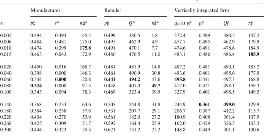
Table 1
Solutions to the`no arrival uncertaintyaproblem withk
v"1,km"1000 (i.e.,m"500),c"0.1 and selecteda-values necessary to
illustrate trends (for each variable or column, the minimum or maximum value is in bold print)
Manufacturer Retailer Vertically integrated"rm
a pH8 rH nHHM pHR QH nRHH kDatpHI pHI QHI nHI E
&
0.002 0.494 0.493 145.4 0.499 380.5 1.8 372.4 0.499 380.5 147.2 1.00
0.006 0.484 0.481 175.0 0.495 462.9 4.9 457.7 0.495 462.9 179.9 1.00
0.010 0.474 0.399 175.8 0.491 470.1 7.7 474.6 0.491 478.6 184.9 0.99
0.015 0.463 0.043 172.9 0.486 476.5 11.0 483.1 0.486 486.4 185.9 0.99
0.020 0.450 0.016 168.7 0.481 481.9 14.8 487.2 0.481 490.1 185.2 0.99
0.040 0.398 0.000 146.3 0.461 490.9 30.8 493.6 0.461 495.6 177.9 0.99
0.060 0.344 0.000 120.8 0.441 494.2 47.6 495.8 0.441 497.3 168.8 0.99
0.080 0.324 0.000 91.3 0.448 407.0 49.7 412.0 0.421 498.1 159.3 0.89
0.100 0.343 0.094 78.3 0.469 323.4 39.9 327.9 0.401 498.5 149.5 0.79
0.140 0.368 0.233 64.6 0.503 244.8 31.8 244.9 0.361 499.0 129.9 0.74
0.180 0.384 0.258 57.8 0.531 207.7 29.1 206.7 0.387 412.2 115.7 0.75
0.220 0.404 0.270 53.9 0.561 182.0 27.2 180.9 0.408 361.4 107.9 0.75
0.260 0.425 0.309 51.7 0.592 164.4 25.9 162.0 0.429 326.5 103.3 0.75
0.300 0.444 0.323 50.3 0.621 151.2 25.2 148.8 0.449 301.1 100.6 0.75
0.400 0.494 0.386 49.3 0.696 131.1 24.7 127.2 0.499 260.0 98.4 0.75
0.480 0.532 0.415 49.7 0.756 120.6 24.9 116.8 0.539 239.5 99.2 0.75
2We investigated the situation of c"0.0 because it is the (only) situation analyzed in detail in [1, Section 4]. This zero-cost situation produces solutions exhibiting special patterns not shared by solutions from situations with c'0. We feel that situations withc'0 are at least as common as a situation with
c"0, and for brevity sake only characteristics shared by`c'0a situations will be reported in this paper.
2.4. Ranges of parameters of numerical solutions obtained in this study
Numerical solutions were obtained for various combinations of the following parameter values: c"0.0}0.42in steps of 0.1;k
v"10n withn"1}3
(see Eq. (15)); k
m"10n with n"3}5; a" 0.005}0.490 in steps of 0.005. Recall thatb"0 in this section. Table 1 presents solutions for the case of: k
v"1, km"1000 (i.e., deterministic m"500), c"0.1, uniform F(v) and selected a-values. Solu-tions were also obtained (not shown) for normal and beta as well as uniform (v)s.
Table 1 and all other tables in this paper are constructed with the following approach: we ascer-tain the patterns of the problem's behavior using
numerical solutions from a large number of di! er-ent combinations of parameter values, a very small subset of these solutions are then tabulated here to illustrate the patterns so ascertained. Thus, the pat-terns we will be generalizing below based on Table 1 have been con"rmed with numerical solutions
from many di!erent combinations of parameter
values andF(v)s.
2.5. Patterns of behavior of the optimal solutions:
Vertically integratedxrm
Start with the case of a"0 (i.e., v"1
2 is now
deterministic) * hence p
R"pI"12 and (buying
probability) P
""12 are "xed. Eq. (6a) gives
k
D"250 andpD"11.18. For the vertically integ-rated"rm, the corresponding formula for Eq. (8) is SLHI"(p
I!c)/pI and QHI"H~1[(SLHI)].
Withc"0.1 as depicted in Table 1, SLH"0.8,z" U~1(0.8)"0.842; hence, QHI"H~1(0.8)"k
D# zp
3For example, ifv&;[0.5!a, 0.5#a] as assumed in MP [1], straightforward manipulations give
kD"mM1![(p
Now considera'0. SubstitutingF(v) from (15b) intoP
"'s de"nition (i.e.,P""1!F(pR)) and di!
er-entiating gives dP
"/dpR"!1/(2akv). That is,
when a is non-zero but very small, a very small
reduction in unit retail price (eitherp
I orpR) leads
to a very large increase in P
" * and hence kD. Therefore, thenHI-column in Table 1 shows that as a"rst becomes non-zero, the initial ability to `ma-nipulate pricesa leads to a rapid rise in nHI. This justi"es the largerQHI, which in turn produces the
increasing nHI. However, as a becomes larger
('0.015 in Table 1), the necessaryp
I-reduction is
not fully compensated by the desirable P
" -in-crement, andnHI `peaks outa. Eventually, whenais too large ('0.14 in Table 1), it is not even worth-while to strive for a highP
" by maintaining a low p
I, andpHI increases.
Note thatnHI ata'0 is never less thannHI"98.4 computed above fora"0. However, the bene"t of a non-zero ato nHI peaks ata"0.015. This non-monotonic e!ect of v'sais largely due to the fact that in MP's (and hence our) model, for a givenp
R,
a change ina(causing a change inP
") causes both k
DandpDto change (see (6a)), and the dependence
betweenk
D's andpD's changes is complex.3A use-ful extension of the current model is to develop a way to specify valuation uncertainty (or a related attribute) such that k
D and pD can be controlled
independently when one changes the valuation-un-certainty magnitude.
2.6. Patterns of behavior of the optimal solutions:
manufacturerversus retailer
For the non-integrated situation, MP showed that under Alternative A, rH"0 always. In con-trast, Table 1 shows that under Alternative B, rHO0 typically.
A more interesting phenomenon is revealed by thenHHR column. Together with the next section, the combined results of this paper will show that the retailer`earns his wayaonlywhen he can: either (i) shoulder the risk of bearing the cost of unsold merchandise; and/or (ii) properly manipulate the retail price (which is beyond the manufacturer's control in the current context). The manufacturer is interested in maximizing his own expected pro"t, which in the current context implies that he isnot interested in sharing his pro"t with the retailer unless he is`forced to do soa.
Therefore, when possible, the manufacturer will choose not to share with the retailer the risk asso-ciated with unsold merchandise, and this is achieved by granting a largerto the retailer. Thus, in the"rst few rows of Table 1, the manufacturer setsrclose top
8, and there is also little retail-price manipulation to be done (sinceais small), hence the retailer's pro"t share (nHHR ) is very small. An impor-tant and counter-intuitive point to note is a large r is often not bene"cial to the retailer at all! If p
8 were "xed (probably a common implicit as-sumption), a largerr is indeed more bene"cial to the retailer. However, ifp
8is variable, then a manu-facturer can often reduce the retailer's pro"t share by matching a larger r with a suitably larger p
8. Section 3 below will illustrate a stronger example of this e!ect for Case 2 (wherevis deterministic).
When one moves down Table 1, the largera(i.e., price manipulability) itself leads to a higher re-tailer's pro"t. At the same time, the desirability of inducing the retailer to order more leads the manu-facturer to: (i) reducep
8, but also (ii) compensate himself somewhat against the reducedp
8by reduc-ingr. Therreduction then also leads to a higher retailer's pro"t. The combination of these two fac-tors bringsnHHR to a peak (at a"0.08 in Table 1).
Towards the bottom of Table 1 (when a is too
large), as was true for the integrated"rm, it is not worthwhile for the `playersa to strive for a high P
" by maintaining a low retail price, hence the manufacturer increases his p
to do, thereforenHRis much higher ata"0.48 than ata"(say) 0.015 (when the ratiorH/pH8 was much lower, i.e., when the retailer gets to bear most of the risk of unsold merchandise). In other words, for the given parameters in Table 1, the risk-bearing pro"t
opportunity for the retailer (due to a low r) at
a"0.015 is less in#uential than the price-manipu-lating pro"t opportunity ata"0.48.
The last column in Table 1 givesE
&de"ned in (1). E& deteriorates as a increases; it is very close to
1 whena is small* the reason for this
phenom-enon will become very clear after Section 3.
3. Case 2: No valuation uncertainty
This section shows how the solution of Case 2 is a!ected when one (in contrast to MP's approach) explicitly addresses the mechanism necessary for the manufacturer to manipulate the retailer's pur-chase-quantity decision. This factor is unrelated to the di!erent interpretations ofvconsidered in Sec-tion 2. In this secSec-tion,v"<(deterministic).
3.1. Summary of MP's statements,approach,results
and summary of our diwerences
With < deterministic, MP stated that the re-tailer's problem is
maxn
R"pR
CP
Qm
xdG(x)#
P
m6
Q
QdG(x)
D
!p
8Q#r
P
Qm
(Q!x) dG(x). (17)
However, in MP's assumed scenario the retailer
never gets to solve this problem because: (i) Case 2 explicitly assumes that p
R"< is "xed by the
market; but (ii) in addition, MP assume that the
retailer will order the QH units prescribed by the manufacturer (see below).
MP [1, p. 697] stated that`In equilibrium... the manufacturer sets r"< and p
8"<... given the manufacturer's choice of
<"rH"pH8, (18)
... the manufacturer's problem (is)a: max
Q nM
"<
CP
Q mxdG(x)#
P
m6
Q
QdG(x)
D
!cQ (19)and solving for `dnM/dQ"0a gives the QH that maximizesnM (notnR) as
QH"G~1[(<!c)/<]. (20)
MP also stated [1, p. 697] that`we assume that the manufacturer can induce the retailer to carry (QH
given in Eq. (20))a. The actual mechanism that could induce the required retailer's behavior was not speci"ed or conjectured.
The basic di!erences between MP's and our re-sults are that, under our approach: (i) pHw di!ers from<(contrasting (18)); instead, c(pH8(<; (ii) rH di!ers from < (contrasting (18)); instead, 0(r(p
8; (iii) an explicit mechanism is given for the retailer to determinehisQHR; (iv) the key to our approach is the explicit consideration of the actual magnitude of the retailer's pro"t (assumed to be 0 in MP's model).
3.2. An explicit mechanism to coordinate the
manu-facturer's and retailer's independent decisions
Consider the following numerical example:
m&;(0, 100), hence G~1(p)"100p;
H
c"1; deterministicpR(or<)"4.
(21)
A useful relationship to remember when
m&;(a,b) is
P
Q mxdG(x)"(Q2!a2)/[2(b!a)]. (22)
Consider"rst an integrated"rm. Eqs. (8), (10) and (22) give (note thatr"0 andp
8"cfor an integ-rated"rm):
SLH"H(QHI)"(<!c)/<; hence
QHI"G~1[(4!1)/4)]"G~1(0.75)"75,
H
(23a)nHI"<
P
QH
m
4Earlier, before proposing (25), we assumed tentatively that the manufacturer wants to induceQHI. It is now clear that this assumption is valid, since the manufacturer could not raise his ownnHHm by having E
&(1. His best strategy is to maximize
nIandE
&, and then to get as big of a cut as possible fromnHI.
Consider now the non-integrated system. If the retailer is allowed to solve hisproblem (Eq. (17))
after the manufacturer sets p
8 and r, then
However, sinceQHI in (23a) brings in the maximum possible system pro"t, we assume tentatively that the manufacturer will want to induceQHRto equate QHI ("75, from (23a)). This can be achieved by settingp8andrto satisfy
(<!p
8)/(<!r)"(<!c)/< or rH"<(pH
8!c)/(<!c). (25)
Eq. (25) comes from combining (23a) and (24), and is identical to (2) due to Pasternack [4].
Consider now the implications of (25). Among the in"nite pairs of feasible (p
8,r)-values satisfying condition (25), assumep
8"3.99, hence (25) gives r"3.98661. Substituting this r into (10) and (22) givesn**R "(4!3.98661)][752/200]"0.375. Sim-ilarly, substituting thisp
8 and rinto (14) and (22) givesnHHM "(3.99!1)]75!3.98661 [(75]0.75)!
(752/200)]"112.125. Note that (nHH
M #nHHR )"
112.5"nHI (see (23b)); i.e.,E
&"1. Realizing this, we could have computednHHM as
nHHM "(nHI!nHHR )"(112.5!0.375) (26)
which is much easier than using (14) and (22) (this is an important point for an easy solution to (32), to be considered in the next subsection).4
However, the manufacturer can increasep
8 fur-ther to 3.999 and still induce the retailer to order QHby granting (according to (25))r"3.998661; then (with the same procedures used in the preceding paragraph)nHHR "0.0375,nHHM "112.4125, and still
E
&"1. The above example illustrates that the
manufacturer can setp
8 as close to<as he wants and yet can induce the`righta behavior from the retailer *a direct result from (2) (due to Paster-nack [4]) and recognized by MP in their Footnote 6. However, what we want to emphasize is that
when p
8K<,nHHR becomes so small that the
re-tailers could not possibly stay in business (unless he receives a "xed `handling feea/unit, which then nulli"es the entire manufacturer/retailer pricing problem under consideration). Recall that a less extreme example of this phenomenon appeared earlier in the"rst few rows of Table 1 whena(i.e., retail-price manipulation opportunity) is very small. In the current section, there is no retail-price manipulation for the retailer to do, and naturally the manufacturer wants to shoulder more risk (which brings higher expected pro"t); hence the very high r (but always slightly lower thanp
8 as required by Eq. (25)). The retailer is left with negli-gible risk, hence neglinegli-gible pro"t.
Both Pasternack and MP assume that the above issue is outside the scope of the problem; instead, we propose below that the problem can be made more meaningful by simply adding a constraint guaranteeing a minimum pro"t that keeps the re-tailer in business.
3.3. Our formulation and solution of the Case-2
`Stochastic-maproblem
Assume now that the retailer will`stay in busi-nessa(or, more realistically,`be willing to carry the producta) only if nHHR *¹ (a minimum target). Thus, the manufacturer's problem is to maximize nHH
M while making sure that`nHHR *¹a. Combining
(10), (14) and (25), this problem can be stated as (where (27c) is a combination of (24) and (25)):
For any random variablexwith distribution func-tionH(x), de"nex's`partial expectationaas E
1(x;H,Q)"
P
Qx
xdH(x). (28)
Eq. (27b) can then be rewritten as
(<!r)E
1(m;G,QH)*¹. Given the discussion in the preceding subsection, it is obvious that for any given¹, the optimum of formulation (27) will occur when (<!r)E
1(m;G,QH)"¹ in (27b), i.e., no more but no less than ¹ is given to the retailer.
Noting thatE
1(m;G,QH) is not a function of ror p
8(see (27c) and (28)), the following solution to (27) can be obtained using (in the order given) (27c), (27b), (25), (23b) and (26):
QH
r"G~1[(<!c)/<], rH"<![¹/E
1(m;G,QHr)],
pH8"c#rH!(rHc/<), (29a)
nHI"<E
1(m;G,QHr), nHHR "¹,
nHHM "nHI!nHHR .
For example, if ¹"56.25, substituting the para-meters in (21) into (29a) gives
QHr"QHI"75, E
1(m;G,QH)"28.125,
rH"2, pH8"2.5, (29b)
nHI"4]28.125"112.5, nHR"56.25"¹,
nHHM "56.25
(to cross-check, (10) gives nHHR "(4!2)] 28.125"56.25"¹). Specifying a di!erent ¹ will lead to di!erent numerical answers in (29b).
We showed above that: (i) p8(<; and (ii) rH(pH8. In contrast, MP's numerical solutions to the same problem are: rH"pH8"4 (by model's de"nition), QHM"75 from (20); nHM"112.5 from (23b) or (19);nHR"0, andQHR"QHM via an
unspeci-"ed mechanism.
3.4. Ewect ofb's(i.e., m's uncertainty)magnitude
With m&;(a,b) in the illustrative problem stated in (21), de"ne m's mean as k
m"(a#b)/2.
Simple manipulations starting from (10) and (22) lead to
nHI"SLH[k
m!bkm(1!SLH)] (SLHandk
mde"ned in (23a) and (15a)). (30) Eq. (30) shows thatnHI decreases asb(m's magni-tude of uncertainty) increases*which is expected, given the classical results (e.g., Leland [10]) on the e!ect of demand uncertainty. However, similar ma-nipulations also give
QHI"k
m#2bkm(SLH!12). (31)
Hence, if SLH'0.5, then QHI increases as b in-creases. This di!ers from the classical results (e.g., in Leland [10]) based onmulti-period products, but is actually a standard phenomenon (see, e.g., Lau and Lau [11]) for asingle-period product considered in this, MP's and related studies.
4. Concluding remarks
4.1. Brief summary
Recall that Table 1 in Section 2 showed that when a is small, nHHR is small and E
&K1. This phenomenon is now clearly explained in Section 3 wherea"0. One may therefore note that a fail-ure to achieve`E&"1ais due to valuation uncer-tainty only.
Given below is a (perhaps over-simpli"ed) sum-mary of the di!erences between MP's [1] and our models:
MP's results Our results Case 1: no arrival
uncertainty
rH"0 rHO0 generally
Case 2: no valuation uncertainty
rH"pH8"< rH(pH8(<
Solutions in Sections 2 and 3 indicate that, when-ever practical, a manufacturer should give return credits to the retailer; however, the return credit should be somewhat less than the original whole-sale price (p
8) paid by the retailer. The solutions also show that, without an additional constraint on minimal retailer's pro"t share, the manufacturer can often devise a price-cum-return-credit scheme such that the manufacturer will reap a larger share of the product-market's pro"t than the retailer. Note that Sections 2 and 3 have considered only
Cases 1 and 2 * in which only one of vor m is
stochastic. Case 3 (in which both v and m are
stochastic) is examined in Lau et al. [12], where it is shown that the above conclusions are also valid for Case 3.
4.2. Extensions
Fruitful extensions include: (i) modeling valu-ation uncertainty such that the mean and standard deviation of market demand do not have to vary together and dependently (stated earlier in Section 2); (ii) an in-depth study of the e!ects of errors in estimatingf(v) andg(m); (iii) considering situations in which the manufacturer and the retailer do not share the same market information.
Appendix A. Solving Eqs.(13)and(14)for the Case-1 problem
For any given (p
8,r)-values, the value ofpHRthat
maximizes nHR(p
R) in (13) was obtained with the
IMSL [13] subroutine UVMGS, which executes
the `golden sectiona search technique. The above
step is imbedded in the function-programn
M(p8,r) (Eq. (14)), which was optimized with the IMSL
subroutine BCPOL*which executes Nelder and
Mead's [14]`simplex methoda. Both UVMGS and
BCPOL are designed for non-smooth functions, and we also executed BCPOL with multiple initial points. This is to eliminate any question about the possible e!ect of function smoothness and unim-odality on the validity of our optimal solutions.
References
[1] H.P. Marvel, J. Peck, Demand uncertainty and returns policies, International Economic Review 36 (1995) 691}714. [2] M. Khouja, The newsboy problem under progressive mul-tiple discounts, European Journal of Operational Research 84 (1995) 458}466.
[3] H.S. Lau, Simple formulas for the expected costs in the newsboy problem, European Journal of Operational Research 100 (1997) 557}561.
[4] B.A. Pasternack, Optimal pricing and return policies for perishable commodities, Marketing Science 4 (1985) 166}176.
[5] L.W. Stern, A.I. El-Ansary, Marketing Channels, Prentice-Hall, Englewood Cli!s, NJ, 1988.
[6] W. Chu, P.S. Desai, Channel coordination mechanisms for customer satisfaction, Marketing Science 14 (1995) 343}359.
[7] V. Padmanabhan, I. Png, Manufacturer's returns policies and retail competition, Marketing Science 16 (1997) 81}94. [8] A.M. Mood, F.A. Graybill, D.C. Boes, Introduction to the
Theory of Statistics, McGraw-Hill, New York, 1974. [9] R.L. Winkler, G.M. Roodman, R.R. Britney, The
deter-mination of partial moments, Management Science 19 (1972) 290}296.
[10] H.E. Leland, Theory of the"rm facing uncertain demand, American Economic Review 62 (1972) 278}290. [11] H.S. Lau, A.H.L. Lau, Some results on implementing
a multi-item multi-constraint single-period inventory model, International Journal of Production Economics 48 (1997) 121}128.
[12] H.S. Lau, A.H.L. Lau, K. Willett, Demand uncertainty and returns policies for a seasonal product*an alternative model, Working Paper, College of Business, Oklahoma State University, 1999.
[13] IMSL, Math/Library and Stat/Library, Visual Numerics, Houston, TX, 1994.