CHAPTER IV RESULT OF THE STUDY
This chapter covers Description of the data, test of normality and
homogeneity, result of the data analyses and discussion.
A. Description of The Data
This section described the obtained data of the effectiveness of using
K-W-L Strategy in teaching reading Descriptive text. The presented data consisted of
Mean, Median, Modus, Standard Deviation and Standard Error.
1. The descriptiondata of Pre-Test Score
The students’ pre test score are distributed in the following table in order
toanalyze the students’ knowledge before conducting the treatment.
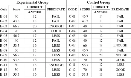
Table 4.1Pre test score of experimental and control group
Experimental Group Control Group
Code Score CORRECT PREDICATE CODE SCORE CORRECT PREDICATE
ANSWER ANSWER
E-01 40 12 FAIL C-01 46.7 14 FAIL
E-02 43.3 13 FAIL C-02 43.3 13 FAIL
E-03 66.7 20 ENOUGH C-03 40 12 FAIL
E-04 70 21 GOOD C-04 40 12 FAIL
E-05 56.7 17 LESS C-05 40 12 FAIL
E-06 40 12 FAIL C-06 40 12 FAIL
E-07 53.3 16 LESS C-07 60 18 ENOUGH
E-08 50 15 LESS C-08 46.7 14 FAIL
E-09 56.7 17 LESS C-09 66.7 20 ENOUGH
E-10 53.3 16 LESS C-10 70 21 GOOD
E-11 60 18 ENOUGH C-11 56.7 17 LESS
E-12 50 15 LESS C-12 70 21 GOOD
E-13 53.3 16 LESS C-13 53.3 16 LESS
E-14 53.3 16 LESS C-14 40 12 FAIL
E-15 50 15 LESS C-15 53.3 16 LESS
E-16 43.3 13 FAIL C-16 50 15 LESS
E-17 66.7 20 ENOUGH C-17 53.3 16 LESS
E-18 50 15 LESS C-18 40 12 FAIL
E-19 40 12 FAIL C19 60 18 ENOUGH
E-20 43.3 13 FAIL C-20 43.3 13 FAIL
E-21 40 12 FAIL C-21 46.7 14 FAIL
E-22 50 15 LESS C-22 40 12 FAIL
TOTAL 1129,9 C-23 40 12 FAIL
AVERAGE 51,4 C-24 53.3 16 LESS
Lowest Score 40 TOTAL 1193,3
Highest Score 70 AVERAGE 49,7
Lowest Score 40
Highest Score 70
The table above showed us the comparison of pre-test score achieved by
experimental and control group students, both class’ achievement are at the same
level. It can be seen that from the students’ score. The highest score 70 and the
lowest score 40, both experimental and control group. It meant that the
experimental and control group have the same level in reading comprehension
before getting the treatment.
a. The Result of Pretest Score of ExperimentalGroup (VII-A)
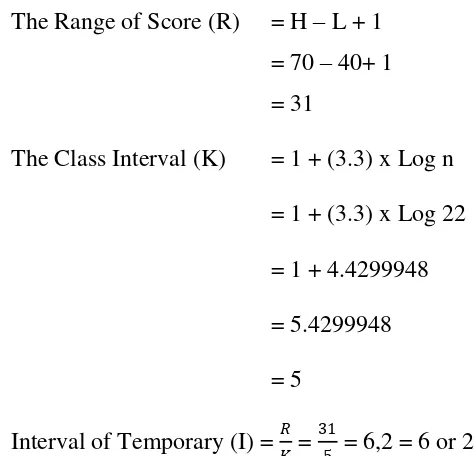
Based on the data above, it was known the highest score was 70 and the
lowest score was 40. To determine the range of score, the class interval, and
interval of temporary,the writer calculated using formula as follows:
The Range of Score (R) = H – L + 1
Table 4.2 Frequency Distribution of the Pretest Score
The distribution of students’ predicate in pretest score of Experimental
group can also be seen in the following figure.
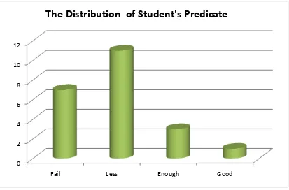
Figure 4.1 The distribution frequency of students’ pretest score for Experimental Group
Figure 4.1 The distribution of students’ predicate in pretest score for Experimental Group
Based on the figure above, it can be seen about the students’ predicate in
pretest score. There were seven students who got Fail predicate. There were
elevenstudents who gotLess Predicate. There were three students who gotEnough
predicate. There was one student who got Good predicate.
The next step, the writer tabulated the scores into the table for the
calculation of mean, standard deviation, and standard error as follows: 0
2 4 6 8 10 12
Fail Less Enough Good
Table 4.3the Table for Calculating Mean, median, modus, Standard deviation. and standard error of Pretest Score.
Class
1) Calculating Mean
= 40.61
4) Standard Deviation
S = 𝑛.∑𝐹𝑋𝑖
standard error of pretest score were 6.29 and 1.37
b. The Result of Pretest Score of ControlGroup (VII-B)
Based on the data pretest score of control group, it was known the
highest score was 70 and the lowest score was 40. To determine the range of
score, the class interval, and interval of temporary,the writer calculated using
Interval of Temporary (I) = 𝑅
Table 4.4 Frequency Distribution of the Pretest Score
Class
The distribution of students’ predicate in pretest score of Control group
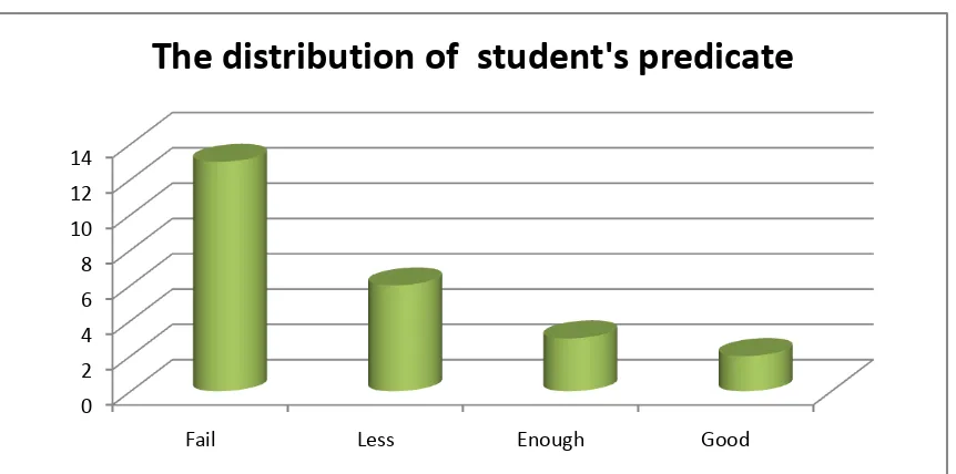
Figure 4.2 The distribution of students’ predicate in pretest score of Control Group
Based on the figure above, it can be seen about the students’ predicate in
pretest score. There thirteenstudents who got Fail predicate. There were
sixstudents who gotLess Predicate. There were three students who got Enough
predicate. There weretwo student who got Good predicate.
The next step, the writer tabulated the scores into the table for the
calculation of mean, median, modus, standard deviation, and standard error as
follows:
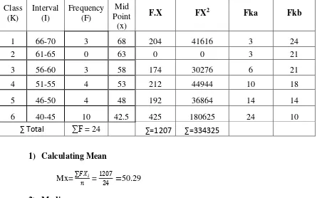
Table 4.5the Table for Calculating Mean, median, modus, Standard deviation. and standard error of Pretest Score of Control group.
Class
1) Calculating Mean
= 39.5 + 107X 5
= 43
3) Modus
Mo = u + 𝑓𝑎
𝑓𝑎+𝑓𝑏 𝑥𝑖
= 39.5 + 6+106 𝑥 5
= 39.5 + 1.87
= 41.37
4) Standard Deviation
S = 𝑛.∑𝐹𝑋𝑖 2− ∑𝐹𝑋
𝑖 2
𝑛 𝑛−1
S = 24.1207− 334325 2
24 24−1
S = 5.38
5) Standard Error
SEmd = 𝑁−𝑆 1=
5.38
24−1= 5.38
4.79 = 1.18
After Calculating, it was found that the standard deviation and the
2. The description data of Post-Test Score
The students’ score are distributed in the following table in order toanalyze
the students’ knowledge after conducting the treatment.
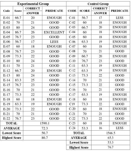
Table 4.6Post-test score of Experimental and Control Group
Experimental Group Control Group
Code Score CORRECT PREDICATE CODE SCORE CORRECT PREDICATE
ANSWER ANSWER
The table above showed us the comparison of post-test score achieved by
experimental and control group students. Both class’ achievement have different
score. It can be seen from the highest score 86.7 and 76.7 and the lowest score
56.7 and 53.3. It meant that the experimental and control group have the different
level in reading comprehension after getting the treatment.
a. The Result of Post-test Score of Experimental Group (VII-A)
Based on the data Post-test score of Experimental group, it was known the
highest score was 86.7 and the lowest score was 56.7. To determine the range of
score, the class interval, and interval of temporary, the writer calculated using
formula as follows:
The Highest Score (H) = 86.7
The Lowest Score (L) = 56.7
The Range of Score (R) = H – L + 1
= 86.7 – 56.7 + 1
= 31
The Class Interval (K) = 1 + (3.3) x Log n
= 1 + (3.3) x Log 22
= 1 + 4.4299948
= 5.4299948
= 5
Interval of Temporary (I) = 𝑅 𝐾 =
31
So, the range of score was 31, the class interval was 5, and interval of
temporary was 6. Then, it was presented using frequency distribution in the
following table:
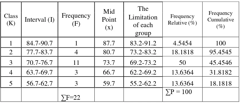
Table 4.7 Frequency Distribution of the Post-test Score
Class
The distribution of students’ predicate in post-test score of Experimental
group.
Figure 4.3 The distribution of students’ predicate in post-test score of Experimental Group
Fail Less Enough Good Exellent
Based on the figure above, it can be seen about the students’ predicate in
pretest score. There was no student who got Fail predicate. There wasone
studentswho got Less predicate. There were fivestudents who gotEnough
Predicate. There were fifteen students who got Good predicate. There was one
student who got Excellent predicate.
The next step, the writer tabulated the scores into the table for the
calculation of mean,median, modus, standard deviation, and standard error as
follows:
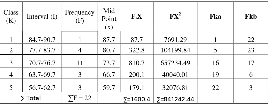
Table 4.8the Table for Calculating Mean, median, modus, Standard deviation. and standard error of Post- test Score.
Class
1) Calculating Mean
= 70.2 +
4) Standard Deviation
S = 𝑛.∑𝐹𝑋𝑖
After Calculating, it was found that the standard deviation and the standard
error of pretest score were 7.74545 and 1.69115
b. The Result of Post-test Score of Control Group (VII-B)
Based on the data Post-test score of control group, it was known the highest
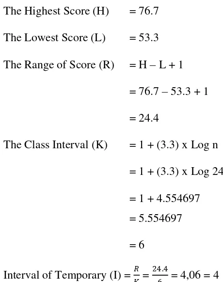
score was 76.7 and the lowest score was 53.3. To determine the range of score,
the class interval, and interval of temporary, the writer calculated using formula as
The Highest Score (H) = 76.7
So, the range of score was 24.4, the class interval was 6, and interval of
temporary was 4. Then, it was presented using frequency distribution in the
following table:
Table 4.9 Frequency Distribution of the Post-test Score
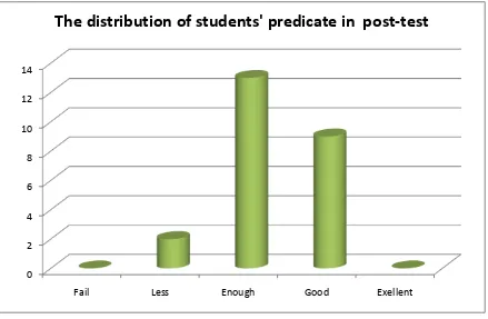
The distribution of students’ predicate in post-test score of Control Group.
Figure 4.4 The distribution of students’ predicate in post-test score of Control Group
Based on the figure above, it can be seen about the students’ predicate in
post-test score. There was no student who got Fail predicate. There were two
studentswho got Less predicate. There were thirteenstudents who gotEnough
Predicate. There were nine students who got Good predicate. There was no
student who got Excellent predicate.
The next step, the writer tabulated the scores into the table for the
calculation of mean,median, modus, standard deviation, and standard error as
follows: 0 2 4 6 8 10 12 14
Fail Less Enough Good Exellent
Table 4.10the Table for Calculating Mean, median, modus, Standard deviation. and standard error of Post- test Score.
Class
1) Calculating Mean
= 58.9667
4) Standard Deviation
S = 𝑛.∑𝐹𝑋𝑖
standard error of pretest score were 6.5925 and 1.37634.
3. The Comparison result of Pre-test and Post-test of Experimental and Control Group
EXPERIMENTAL GROUP CONTROL GROUP
15 E-15 50 76,7 26,7 15 C-15 53,3 73,3 20
16 E-16 43,3 70 26,7 16 C-16 50 70 20
17 E-17 66,7 73,3 6,6 17 C-17 53,3 63,3 10
18 E-18 50 60 10 18 C-18 40 60 20
19 E-19 40 63,3 23,3 19 C-19 60 73,3 13,3
20 E-20 43,3 73,3 30 20 C-20 43,3 60 16,7
21 E-21 40 70 30 21 C-21 46,7 70 23,3
22 E-22 50 76,7 26,7 22 C-22 40 73,3 33,3
TOTAL 1129,9 1590,1 460,2 23 C-23 40 60 20
MEAN 51,4 72,3 20,9 24 C-24 53,3 53,3 0
LOWEST 40 56,7 TOTAL 1193,3 1566,5 373,2
HIGHEST 70 86,7 MEAN 49,7 65,3 15,6
LOWEST 40 53,3
HIGHEST 70 76,7
From the table above the mean score of pre test and post test of the
experimental group were 51,4 and 72,3. Meanwhile, the highest score pre test and
post test of the experimental group were 70 and 86,7, the lowest scores pre test
and post test of the experimental group were 40 and 56,7. In addition, the mean
score pre test and post test of the control group were 49,7 and 65,3. Meanwhile,
the highest score pre test and post test of the control group were 70 and 76,7. The
lowest scores pre test and post test of the control group were 40 and 53,3. Based
on the data above, the difference of mean score between experimental and control
B. Testing of Normality and Homogeinity 1. Normality Test
a. Testing normality of pre-test experimental and control group
Table 4.11 Testing normality of pre-test experimental and control group Tests of Normality
Group
Kolmogorov-Smirnova Shapiro-Wilk
Statistic Df Sig. Statistic df Sig.
Scores
experiment
group
,142 22 ,200* ,920 22 ,676
control group ,168 24 ,076 ,863 24 ,114
The table showed the result of test normality calculation using SPSS 21.0
program. To know the normality of data, the formula could be seen as follows:
If the number of sample. > 50 = Kolmogorov-Smirnov
If the number of sample. < 50 = Shapiro-Wilk
Based on the number of data the writer was 46 < 50, so to analyzed normality
data was used Shapiro-Wilk. The next step, the writer analyzed normality of data
used formula as follows:
If Significance > 0.05 = data is normal distribution
If Significance < 0.05 = data is not normal distribution
Based on data above, significant data of experiment and control group used
Shapiro-Wilk was 0.676 > 0.05 and 0.114 > 0.05. It could be concluded that the data
was normal distribution.
Table 4.12Testing normality of post-test experimental and control group Tests of Normality
Group
Kolmogorov-Smirnova Shapiro-Wilk
Statistic df Sig. Statistic df Sig.
Scores experiment group .122 22 .200* .971 22 .744
control group .174 24 .058 .933 24 .115
The table showed the result of test normality calculation using SPSS 21.0
program. To know the normality of data, the formula could be seen as follows:
If the number of sample. > 50 = Kolmogorov-Smirnov
If the number of sample. < 50 = Shapiro-Wilk
Based on the number of data the writer was 46 < 50, so to analyzed normality
data was used Shapiro-Wilk. The next step, the writer analyzed normality of data
used formula as follows:
If Significance > 0.05 = data is normal distribution
If Significance < 0.05 = data is not normal distribution
Based on data above, significant data of experiment and control group used
Shapiro-Wilk was 0.744 > 0.05 and 0.115 > 0.05. It could be concluded that the data
2. Homogeneity Test
a. Testing Homogeneity of pre-test experimental and control group
Table 4.13Testing Homogeneity of pre-test experimental and control group
Homogeneity Test
Levene's Test for
Equality of
Variances
t-test for Equality of Means
F Sig. T Df Sig.
(2-The table showed the result of Homogeneity test calculation using SPSS 21.0
program. To know the Homogeneity of data, the formula could be seen as follows:
If Sig. > 0,01 = Equal variances assumed or Homogeny distribution
If Sig. < 0,01 = Equal variances not assumedor not Homogeny distribution
Based on data above, significant data was 0,393. The result was 0,393 > 0,01,
it meant the t-test calculation used at the equal variances assumed or data was
b. Testing Homogeneity of post-test experimental and control group
Table 4.14Testing Homogeneity of post-test experimental and control group
Homogeneity Test
Levene's Test for
Equality of
Variances t-test for Equality of Means
99% Confidence
Interval of the
Difference
F Sig. t df
Sig.
(2-tailed)
Mean
Difference
Std. Error
Difference Lower Upper
Scores Equal variances
assumed
.607 .440 3.352 44 .002 7.00644 2.09010 1.37931 12.633
57
Equal variances
not assumed
3.320 40.219 .002 7.00644 2.11064 1.29985 12.713
03
The table showed the result of Homogeneity test calculation using SPSS 21.0
program. To know the Homogeneity of data, the formula could be seen as follows:
If Sig. > 0,01 = Equal variances assumed or Homogeny distribution
If Sig. < 0,01 = Equal variances not assumedor not Homogeny distribution
Based on data above, significant data was 0,440. The result was 0,440 > 0,01,
it meant the t-test calculation used at the equal variances assumed or data was
C. The Result of Data Analysis
1. Testing Hypothesis Using Manual Calculation
Table 4.15 The Standard Deviation and the Standard Error of Experiment and Control Group
Group Standard Deviation Standard Error
Experimental Group 7.74545 1.69115
Control Group 6.5925 1.37634
The table showed the result of the standard deviation calculation of
Experiment group was 7.74545and the result of the standard error was 1.69115.
The result of thestandard deviation calculation of Control group was 6.5925 and
the result of standard error was 1.37634. To examine the hypothesis, the writer
used the formula as follow:
t
observed=
𝑀1−𝑀2
𝑆𝐸𝑚1−𝑆𝐸𝑚2
=
7.74545−6.59251.69115−1.37634
=
1.152950.31481= 3.663
df = (N1 + N2 – 2)
= 22+24-2
a. Interpretation
The result of t – test was interpreted on the result of degree of freedom to get
the ttable. The result of degree of freedom (df) was 44. The following table was the
result of tobserved and ttable from 44 df at 5% and 1% significance level.
Table 4.16 The Result of T-Test Using Manual Calculation
t-observe
t-table
Df 5 % (0,05) 1 % (0,01)
3.663 2.021 2.704 44
The interpretation of the result of t-test using manual calculation, it was found
the tobserved was higher than the ttable at 5% and 1% significance level or 3.663 > 2.021,
3.663 > 2.704. It meant Ha was accepted and Ho was rejected. It could be interpreted
based on the result of calculation that Ha stating that K-W-L strategy was effective
for Teaching Reading Comprehension of the seventh grade students at SMP
Al-Amin Palangka Raya was accepted and Ho stating thatK-W-L strategy was
not effective for Teaching Reading Comprehension of the seventh grade
students at SMP Al-Amin Palangka Raya was rejected. It meant that teaching
reading with K-W-L Strategy Toward Reading Comprehension for the seventh
grade students at SMP Al-Amin Palangka Raya gave significant effect at 5% and
1% significance level.
2. Testing Hypothesis Using SPSS 21.0 Program
The writer also applied SPSS 21.0 program to calculate t – test in testing
the manual calculation of t – test. The result of t – test using SPSS 21.0 program
could be seen as follows:
Table 4.17 Mean, Standard Deviation and Standard Error of experiment group and control groupusing SPSS 21.0 Program
Group Statistics
Group N Mean Std. Deviation Std. Error Mean
Scores experiment group 22 72.2773 7.86032 1.67583
control group 24 65.2708 6.28597 1.28312
The table showed the result of mean calculation of experiment groupwas
72.2773, standard deviation calculation was 7.86032, and standard error of mean
calculation was 1.67583. The result of mean calculation of control groupwas
65.2708, standard deviation calculation was 6.28597, and standard error of mean
was 1.28312.
Table 4.18 The Calculation of T – Test Using SPSS 21.0
Independent Samples Test
Levene's Test for
Equality of
Variances t-test for Equality of Means
99% Confidence
Difference Lower Upper
Scores Equal variances
The table showed the result of t – test calculation using SPSS 21.0 program.
To know the variances score of data, the formula could be seen as follows:
If Sig. > 0,01 = Equal variances assumed
If Sig. < 0,01 = Equal variances not assumed
Based on data above, significant data was 0,440. The result was 0,440 > 0,01,
it meant the t-test calculation used at the equal variances assumed. It found that the
result of tobserved was 3.352, the result of mean difference between experiment and
control group was 7.00644, and thestandard error difference between experiment and
control group was 2.09010.
a. Interpretation
The result of t – test was interpreted on the result of degree of freedom to get
the ttable. The result of degree of freedom (df) was 44. The following table was the
result of tobserved and ttable from 44 df at 5% and 1% significance level.
Table 4.19 The Result of T-Test Using SPSS 21.0 Program
t-observe
t-table
Df 5 % (0,05) 1 % (0,01)
3.352 2.021 2.704 44
The interpretation of the result of t-test using SPSS 21.0 program, it was
found the tobserved was higher than the ttable at 5% and 1% significance level or 3.352 >
2.021, 3.352 > 2.704. It meant Ha was accepted and Ho was rejected. It could be
interpreted based on the result of calculation that Ha stating that K-W-L strategy
students at SMP Al-Amin Palangka Raya was accepted and Ho stating that
K-W-L strategy was not effective for Teaching Reading Comprehension of the
seventh grade students at SMP Al-Amin Palangka Raya was rejected. It meant
that teaching reading with K-W-L Strategy Toward Reading Comprehension for
the seventh grade students at SMP Al-Amin Palangka Raya gave significant
effect at 5% and 1% significance level.
D. Discussion
The result of analysis showed that there was significant effect of K-W-L
strategy Toward Reading Comprehension forthe seventh grade students at
SMP Al-Amin Palangka Raya.The students who were taught used K-W-L
strategyreached higher score than those who were taught without used
K-W-L strategy.
Meanwhile, after the data was calculated using manual calculation of ttest.It
was found the tobserved was higher than the ttable at 5% and 1% significance level or
3.663 > 2.021, 3.663 > 2.704. It meant Ha was accepted and Ho was rejected. And the
data calculated using SPSS 21.0 program, it was found the tobserved was higher than
the ttable at 5% and 1% significance level or 3.352 > 2.021, 3.352 > 2.704. It meant Ha
was accepted and Ho was rejected. This finding indicated that the alternative
hypothesis (Ha) stating that there was any significant effect of K-W-L strategy
Toward Reading Comprehension for the seventh grade students at SMP
Al-Amin Palangka Raya was accepted.On the contrary,the Null hypothesis (Ho)
stating that there was no any significant effect of K-W-L strategy Toward
Palangka Raya was rejected.Based on the result the data analysis showed that
using K-W-L Strategy gave significance effect for the students’ reading
comprehension scores of Seventh grade students at SMP Al-amin Palangka Raya.
After the students have been taught by using K-W-L Strategy, the reading
score were higher than before implementing K-W-L Strategy as a learning
strategy. It can be seen in the comparison of pre test and post test score of
experimental group and control group (See p.61). This finding indicated that
K-W-L strategy was effective and supports the previous research done by Zhang
Fengjuan, Eviani Damastuti and Anne Crout Shelleythat also stated teaching
reading by using K-W-L strategy was effective.
There were some reason why using K-W-L Strategy gave significance effect
for the students’ reading comprehension scores of Seventh grade students at SMP
Al-amin Palangka Raya.First, K-W-L Strategy was effective in terms of
improving the students’ English reading score. It can be seen from the
improvement of the students’ score average in the post-test. From the mean
score of control and experiment were 72.3 and 65.3. (See p.62).It supports the
previous study by Eviani Damastuti and Sugini states that using K-W-L strategy
increase in reading ability significantly intensified.
It was suitable withthe result of pre-test and post test for Experiment and
control Group. (See p.44). In the pre-test of experiment group there wereseven
students that got fail predicate. They were E-01, E-02, E-06, E-16, E-19, E-20 and
E-21. There were eleven students that got less predicate. They were E-05, E-07,
students that got enough predicate. They are E-03, E-11 and E-17. There was one
student that got good predicate. She was E-04. Then, in the pre-test score of
control group there were thirteen students that got fail predicate. They were C-01,
C-02, C-03, C-04, C-05, C-06, C-08, C-14, C-18, C-20, C-21, C-22 and C-23.
There were six students that got less predicate. They were 11, 13, 15,
C-16, C-17 and C-24. There were three students that got enough predicate. They
were C-07, C-09 and C-19. There were two students that got good predicate. They
were C-10 and C-12.
Based on the result of post-test for experimental and control group, (See
p.53). In the experimental group, there was no student that got in fail predicate.
There was one student that got less predicate, he was E-06. There were five
students that got enough predicate. They were E-01, E-07, E-12, E-18 and E-18.
There were fifteen students that got good predicate. They were E-02, E-03, E-05,
E-08, E-09, E-10, E-11, E-13, E-14, E-15, E-16, E-17, E-20, E-21 and E-22.
There was one student that got excellent predicate, she was E-04. In the control
group, there was no student that got in fail predicate. There were two students that
got less predicate. They were C-01 and C-24. There were thirteen students that got
enough predicate. They were 02, 03, 04, 05, 06, 07, 09, 11,
C-12, C-17, C-18, C-20 and C-23. There were nine students that got good predicate.
They were C-08, C-10, C-13, C-14, C-15, C-16, C-19, C-21 and C-22.
The next reason wasK-W-L strategycan motivate students in teaching
learning process. It was suitable with the students response when learning process
topic with their background knowledge. It was necessary to keep responses inside
the topic. It indicated that using K-W-L strategy was effective in enhance reading
motivation and encouragement. (See appendix 6). It supports with Ferdinand
Nicholas Boonde states that K-W-L strategycan motivate the students to take a
part in the teaching learning process and Filling the columns is effective to help
the students understand the reading text.
The last reason was K-W-L strategy gave the students can answer both
literal and inferential reading comprehension types. It indicated the test was
suitable for junior high school student (see appendix4). It supports with Zhang FengjuanK-W-L strategy is an instructional scheme that develops active reading of descriptive texts by activating learners’ background knowledge.
Those are the result of pre-test compared with post-test for experimental
group and control group of students at SMP Al-Amin Palangka Raya. Based on
the theories and the writer’s result,K-W-L Strategy gave significance effect for the
students’ reading comprehension scores of Seventh grade students at SMP