Portfolio Theory to Obtain Best Weighting Structure
Tumpal Sihombing*
Bond Research Institute
The world is entering the era of recession when the trend is bearish and market is not so favor-able. The capital markets in every major country were experiencing great amount of loss and people suffered in their investment. The Jakarta Composite Index (JCI) has shown a great downturn for the past one year but the trend bearish year of the JCI. Therefore, rational investors should consider restructuring their portfolio to set bigger proportion in bonds and cash instead of stocks. Investors
can apply modern portfolio theory by Harry Markowitz to find the optimum asset allocation for their portfolio. Higher return is always associated with higher risk. This study shows investors how to find
out the lowest risk of a portfolio investment by providing them with several structures of portfolio weighting. By this way, investor can compare and make the decision based on risk-return consider-ation and opportunity cost as well.
Keywords: Modern portfolio theory, Monte Carlo, linear programming
Introduction
The crisis was first triggered by the sub-prime mortgage issues in the US financial mar-ket. At that time (over and about year 2006-2007), some people and organizations might actually have already been aware regarding the latent problems of sub-prime mortgage prior
to the current crisis that the world is now fac
-ing. US investment banking industry has failed and collapsed. The financial crisis has become
one of the most radical reshaping of the global
banking sector. Meanwhile, governments and the private sector battle to shore up the financial system, following the disappearance of
Leh-man and Merrill as independent entities and the billions of dollars government rescue of AIG.
The housing market in US is related to the
mortgage industry in significant term. And at that time, investment bankings were mainly
invest the fund into the mortgage-backed rities, issued by some institutions which secu-ritize the mortgage into MBS. This is one of the investment vehicle that eventually has hurt the
investors. There are lots of varieties of instru -ments available in the market. Allocating all
the funds into single instrument is significantly vulnerable to risk (Bodie, Kane, and Marcus, 2008). Otherwise, putting funds partially into more than one instrument may distribute the
risk of investing as well as the return itself. Re -turn is the proceeds gained from the willingness
to take the risk (Damodaran, 2002). The higher the risk, the higher the potential gain in return.
The way in allocating the funds into some
available instruments of investment is the basis
of effective diversification in portfolio manage-ment. Diversification is a powerful method to manage investment risk. While diversification is good, certain types of diversifications are
bet-* Menara Global 17th Floor Suite A, Jl. Jend. Gatot Subroto Kav. 27, Jakarta 12950, Indonesia. E-mail:
ter. This was the premise of Harry Markowitz’s Nobel Prize winning theory. He showed that
when the assets in a portfolio do not move in
concert with each other, their individual risks can be effectively diversified away (Gibson, 1996). Diversification among assets that move together is ineffective diversification. Effective diversification reduces portfolio volatility and smoothes out the returns. In general, anything that reduces volatility eventually increases the
compound rate of returns.
Effective diversification can be done through
an effective asset allocation. Asset allocation is an investment method that pools or combines
various asset classes such as stocks, bonds, and
cash in a single portfolio of investment. It has to wise in terms of risk and return on portfolio in
-vestment in order to have an effective diversifi-cation. Back to the above example, conducting such allocation may move the investor away
from the effective assets allocation and pos
-sibly even expose the investor to more risk if the pool of assets was not well-diversified since the first time. If that is the case, then it is the
time the conservative investors should step in and bring the portfolio into the effective diver
-sification. They should change the allocation,
in other words consider the asset rebalancing. There are some methods on portfolio rebalanc
-ing (Fischer and Jordan, 1991), such as:
• Buy-and-hold. It is a do-nothing strategy after buying some assets. This strategy comprises of initial weights allocation and followed by
no action forever.
• Constant-mix. It is a strategy to dynamically rebalance the current weightings by trading
whenever market conditions have changed
from the first balance. It implies a constant
proportion of the portfolio invested in shares.
• Constant proportion portfolio insurance. This strategy involves buying shares as they rise and selling them as they fall. When imple-menting the strategy, investors select a floor
below which the portfolio value is not al -lowed to fall to certain level.
• Active tactical. The goal is to outperform the constant-mix strategy by overweighting asset
classes that are expected to be outperformed whereas underweight sectors that are expect
-ed to be underperform-ed. This strategy allows investors to flexibly follow elements of the constant-mix and constant proportion
strate-gies based on market context.
• Black-Litterman. In this model, investor in-puts any number of views or statements about the expected returns of arbitrary portfolios,
and the model combines the views with equi
-librium, producing both the set of expected
returns of assets as well as the optimal port -folio weights. The investor should invest in
portfolio first, and then rebalance from current weighting by adding some weights on port-folios representing investor’s views (Vince, 1990).
As time goes by, many strategies or ap-proaches have been improved lately by using advanced knowledge and know-how related to the portfolio risk in terms of investment and fi-nance area (Bodie, Kane, and Marcus, 2008).
There are some approaches that have been
known as tools to better the investor’s decision
when dealing with the uncertain future events
or market volatility, they are:
• Altman Z-Score. This model was created by Edward Altman. It combines some financial ratios to determine the possibility of bank-ruptcy of a company in certain industry. The lower the score, the higher the probability of bankruptcy.
• Black Scholes. It was developed at 1973 by Fisher Black, Robert Merton and Myron Scholes, and is still applied today as one al-ternative way of determining fair prices of
options. This model assumes that market is
efficient, European exercise terms apply, and
that interest rates should remain constant and known.
• Binomial model. It is an equation or an
open-form that generates a tree of possible future price movements. The performance of a port
-folio is measured by the result of investor’s strategy compared to a certain benchmark selected. Any relationship between investors’
There are three main issues in this research
as listed below :
• What kinds of asset should be preferred or
se-lected from some asset classes available in the onshore capital market of Indonesia consider -ing recent market situation?
• How should all the funds be allocated amongst
the structured weightings into those selected assets in order to have the possible lowest risk
in the future without significantly
jeopardiz-ing the portfolio rate of return?
• What portfolio weight structure should be se-lected in order to satisfy the investor’s
objec-tives and constraints or requirements based on the historical and recent market situation?
Literature Review
Portfolio management
Portfolios are combinations of assets, they
consist of set of securities or asset classes (Fis
-cher and Jordan, 1991). Conventional portfolio
planning called for the selection of those assets
that best fit the investor needs and desires. Oth-erwise, modern portfolio theory suggests that the traditional approach to portfolio analysis, selection and management may well yield less
than optimum result. Portfolio management is the process of maintaining and allocating set of
assets to meet the investment objectives of
in-vestor.
Monte Carlo in Finance
The Monte Carlo approach can be utilized to
obtain solutions to quantitative problems which
need forecast and simulation. Monte Carlo
ap-proach can provide an optimal solution to an
optimization problem by directly simulating
the process and then calculating the statistics
results. Monte Carlo simulation is a method
for evaluating a model using sets of random
numbers as inputs. Monte Carlo approach is often utilized when the model is complex and
involves massive uncertain parameters. A simu -lation can be done and evaluate in a massive
number of runs by using computer’s proces-sor. Monte Carlo simulation generates random
numbers from certain type of distributions,
generates those numbers and stores the model outcomes. This process is then being repeated
many times before the results are displayed as
a new combined distribution. The general ap
-proach of Monte Carlo Simulation can be
de-scribed in Figure 1.
This process can be actually be done in more descriptive, mathematical, or algorithmic way, but the principle of conducting Monte Carlo simulation is just similar to the flowchart in Figure 1. Defining a domain of possible inputs
is one of the input parts which are determined
by the investor. In this case, it may come to
de-cision of investor regarding the portfolio weight
selection in order to have effective
diversifica-tion. The next step will deal with generating random number with certain predetermined
type of distribution. In this research the large
number of expected returns will be generated in the basis of uniform distribution.
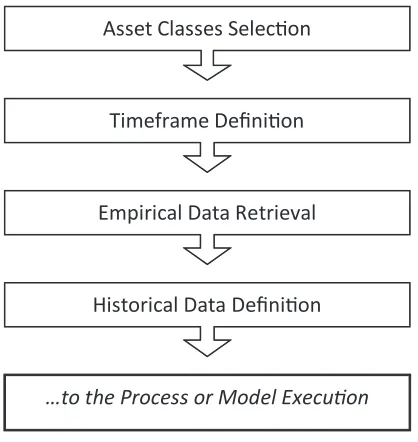
Research Method
Basic framework
Managing investment portfolios is a dynam-ic and an ongoing process. It consists of many steps such as specifying the investor’s invest-ment objectives and constraints, developing investment strategies, evaluation of portfolio composition and performance, monitoring in-vestor and market conditions, and finally im-plementing any necessary rebalancing (Fischer and Jordan, 1991). In general, the very basis of those steps can be described by Figure 2.
Model requirement
In an optimization model, there should be input and constraints definition in purpose to meet the model objective. The input can be de-fined by the investor together with the empirical
data prior to the model execution.
Historical data
This can be done if the assets have been defined and the timeframe as well, to mention also the importance of the availability of empirical data of each asset in the market. Therefore, even in the input stage, the constraints have already
been applied to the model. Figure 3 is the input
side of the graph-based model representation: In the historical data definition, there will 12 assets (nine stocks, two bonds, one cash) with 36 month of historical net earnings data for
each asset.
Data preparation
Data preparation is part of the historical data
definition. But rather than merely taken from the certain sources, those are data which have
already been statistically calculated prior to the
model execution. There are two tasks needed to
be done in this part. The first task is to have the three years historical monthly net earnings of
each asset selected. The second task is to have
the statistically-related data based on the results obtained from the first task.
Maximum and minimum data are needed in purpose to generate the random data based on uniform distribution. The reason for this is to
have the same probability of the value which may exist in the future from the large number of runs simulated later (Levin and Rubin, 1998).
The mean average and standard deviation are
actually generated in order to compare to the figures obtained from the outcomes of optimi-zation and simulation in the next phase of this
Figure 1. General flow of Monte Carlo simulation
research. The mean return used is the arithmetic
average for the sake of simplicity in the
calcu-lation and the relevance as well. The standard
deviation for each asset is calculated by using the standard routine function in the Excel-based tool as a representation of volatility of each
as-set in the past.
Model objective
Generally there are two types of objectives in the optimization model, they are maximiza-tion and minimizamaximiza-tion. The first one needed to be maximized is usually the expected return
of the portfolio whereas the portfolio risk is to
be minimized. Therefore, the investors need to
aware and also ought to select which of both
main objectives fit preference of investor.
Usu-ally the investor will fall to the final portfolio
which has the highest return with the lowest
risk possibly constructed. This is the challenge of the portfolio management actually.
Lowest portfolio risk
Lowest portfolio risk is the possible mini-mum of volatility or standard deviation that can be reached from certain diversification or
portfolio weight structure. The portfolio weight
structures are going to be defined in the
con-straints part of the model.
The calculation of portfolio risk needs only two sets of data, they are the portfolio weight
structures and the portfolio variance. The port -folio expected returns data is nothing to do with the process of calculating the portfolio risk.
Figure 3. Historical data filtering
Since it only deals with the portfolio risk, then at this part the minimization is the only task needed to be done. The model aims at finding the lowest portfolio risk possible from
adjust-ing the weight structure. This is the part of the process in the portfolios selection.
Since no investor will know what will hap
-pen in the future, then the most rational thing to do is trying to obtain the weight structure that
will have the lowest portfolio risk that can be reached.
Highest portfolio expected return
The portfolio expected return is simply cal-culated by the multiplication of weighting to
the expected return of each asset selected. The expected returns of each asset are a function of random in uniform distribution. Since there will
be many weighting structures involved in the
model as well as the random expected returns
of portfolio, then there will be many portfolio
expected returns that will be populated from the process.
Objective selection
The main part of the first phase of this model is the process minimizing the portfolio risk for every weighting structure defined in the con-straints part of the model definition. It is the risk that is needed to be minimized prior to the
simulation of the random expected returns pos
-sibly constructed in the uniform distribution. The principle objective of this model is actually
to have a single weighting structure which is
statistically able to provide investors with the
maximum portfolio rate of return on investment with the lowest risk based on the forecasted ex -pected returns of each asset.
Model constraint
There are boundaries in the process of op
-timization that the model should be subjected
to. Those are set to limit the process in order to
have the single solution at the final stage of the
model.
Basic constraint
The basic constraint is applied to certain parameter in the model. In this research were applied to the weighting of portfolio construct
-ed. In mathematical expression, the basic con-straints are defined as below:
1)
where,
w
i ≥ 0 where i = 1,2,3,4,…n and i is integer; wi = the series of weight structure;
n = number of assets.
Total constraints
The basic and conditional constraints are combined together prior to the execution of the model. These are the whole constraints applied
as the boundaries the model is subjected to: • Maximum and minimum value of expected
return;
• Uniform distribution of random number
generation;
• Total random series generated = 10,000; • Total shares of in portfolio weight = 100%; • Each of shares of weight is at minimum 0%
and maximum 100%;
• The 17 weighting structures as conditional
constraints;
• Minimum target return, in this research is set about 18% p.a. or 1.5% p.m.
All the constraints above should be applied
in AND method instead of OR. It means the so-lution should satisfy each of the constraints and
not even single constraint is violated.
Model format
This is how the model is shown in a descrip
-tive way to reach the objec-tive of investor. The objective is to find the optimal or best
weight-ing structure with the lowest risk possible in or
-der to deal with the uncertainty of future event by utilizing the defined historical data and
the model is going to be executed. The basic and conditional constraints are applied into the historical input and investors preference (in this
case the 17 weighting structures of portfolio as results of optimization). The next stage of the model is to simulate the outcomes by using the defined weighting structures and random expected returns and statistically analyzed the result. Each result will have different charac-teristic and proximity to the solution needed.
The selected portfolio should be the one with the lowest portfolio risk but with the expected return that is equal or greater than target return
defined by the investor since the first time.
Result and Discussion
Data input
There are two types of relevant data for this research, first is the historical data which com-prises the empirical data of asset’s net earnings from the past three years in monthly period, and the second is the statistical-based data which comprises parameters such as mean or average, standard deviation, covariance, coefficient of correlation, and else.
Asset picking
The analytical components that most com-monly utilized by equity investors to select
good investment prospects might include some
or many categories (Fischer and Jordan, 1991). Industrial or sector analysis may involve iden-tification and analysis of various variables in the economy that are likely to gain superior
performance. Scholars indicate that the health
of an asset in particular sector or industry is as
important as the performance of the individual
asset itself. In other words, even the best asset located in a weak sector will probably may per-form poorly because that sector is out of favor
or some assets looked like bullish but eventu
-ally bearish instead. Each sector or industry is unique in terms of its customer base, market share among firms, industry growth, competi-tion, regulacompeti-tion, and business cycles (Baumohl, 2008).
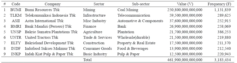
There are three types of empirical data in-volved in the research, they are from equity market (represented by selected stocks), fixed income market (represented by selected gov-ernment and corporate bonds), and money mar-ket (single instrument of cash). The list is taken from LQ-45 population list. Those stocks are considerably leading the industries in terms of liquidity and volume of trading. All the stocks in the population were categorized into nine sectors. Therefore, there should be nine rep-resenting top stocks taken from LQ-45 list of
stocks.
Based on the volume and frequency together
(which was stated as V x F in terms of math -ematic as stated in the header part of last col
-umn), the nine top representing stocks should
be BUMI, TLKM, ASII, BMRI, UNSP, UNTR, ELTY, INDF, and INKP. Those stocks respre-sents stocks of the industry of mining, infra-structure, miscellaneous, finance and banking, agriculture, trade and services, construction, consumer goods, and basic industry, respec-tively.
Bonds are another instruments included in
the portfolio investment. There are two types of bonds included in this research, government bond and corporate bond. FR00002 represents the government bond and HMSP03 (HM Sam-poerna corporate bond) represents corporate
bonds.
There are some reasons behind the selec -tion of both bonds in this research. First is the
liquidity. The maturity of FR00002 is near, which will be matured in year 2009. It made this bond easy to transact and liquid in fixed-income market. The second is coupon-bearing bond type. FR00002 is one of the bonds with
highest coupon available in current Indonesia
fixed-income market. It has 14% gross cou-pon rate per year, and it is the top government bond instrument in the fixed-income market in
terms of coupon rate with length of tenure less
than one year. The third is the data availability. FR00002 has already traded in the market for more than three years. Therefore, the historical data are available to be retrieved and analyzed
together with other instruments involved in this
research. The corporate bond is represented by HMSP03, stands for HM Sampoerna Corporate Bond. Rating-wise, bond is considered to be in
the level of investment grade.
For money market instrument, this research only uses the government-issued money market, it is called SBI (Bank of Indonesia Certificate).
Table 1. List of selected stocks out of LQ-45
# Code Company Sector Sub-sector Value (V) Frequency (F)
The terms of the SBI used in this research was
one month, therefore the name is SBI 1-month. The reason behind this was purely based on the total market demand for this SBI 1-month
which considered as the biggest amongst all
SBIs available in the money market. This can be seen at Table 2 that mentioned SBI 1-month
as the cash instrument with the highest absorbed
amount at year-end 2008.
Historical timeframe
It needs three years of monthly historical data of asset’s net earnings for the research to complete the analysis and evaluation prior to
obtaining the best and expected result. Three
years backward can exhibit roughly three kind
of world economic conditions which was total
-ly different. By ana-lyzing the world economic data (especially for total GDP or world output), it is obvious that the Y2006 was an uptrend year, Y2007 was a bullish year, Y2008 was the
top of the peak and also the beginning of reces
-sion era, as shown by Table 3.
National Bureau of Economic Research (NBER) of US has declared that United States had been in recession in year 2008 and several economists expressed that recovery may not
appear until as late as 2011 (Foldvary, 2007). It means that the year 2008 is the starting point of the recession cycle as explained above. That completes the recovery-bullish-recession cy-cles of the economy, thus completes the three
economic condition of the world. That is the
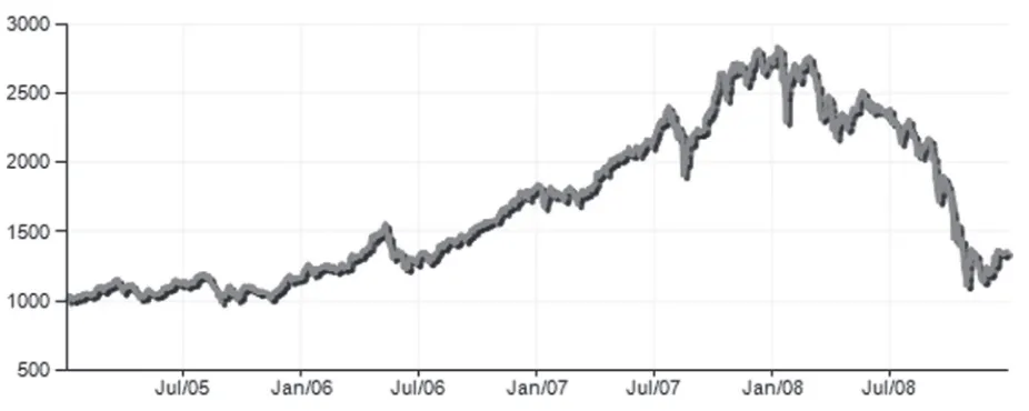
reason behind the three years historical data re-trieval that will be utilized as the main input of the model. If the world is definitely in reces-sion, the question remains whether Indonesia has already been in recession also. While this research is being conceived, the government of Republic of Indonesia has not yet clearly de-clared that Indonesia already in recession al-though the world had has. Nevertheless, regard-less Indonesia has already entered the recession cycle or not, one thing should be considered is the pattern of capital market cycle in Indone-sia. JCI (Jakarta Composite Index) represents the price movement of total equity in Indonesia capital market. This JCI movement is closely related to the movement of GDP in certain way
since it comprises hundreds of vital companies within it.
JCI vehicle comprises more than 300
com-panies and have strong relationship with the
Indonesia Gross Domestic Product (GDP). At a glance, it can be analyzed that from the year
Table 2. Auction result of SBI dan SBIS at 31st December 2008
Parameters of instruments SBI SBIS
Tenor 24 87 178 28
Overall indicative target 57.5
Received offer 44.3 4.45 6.1 0.92
Range of bid rate 9.25% - 11.25% 11.00% – 11.20% 11.70% - 12.00%
-Absorbed amount 29.48 3.59 5.46 0.92
Stop of rate 10.90% (FA) 11.15% (FA) 11.90% (FA)
-Weighted average SBI's auction 10.83 11.08474 11.82
-Return of SBIS - - - 10.83381
Settlement date 5-Jan-09 5-Jan-09 5-Jan-09 31-Dec-08
Due date 29-Jan-09 2-Apr-09 2-Jul-09 28-Jan-09
Frequency of auction 184 27 26 16
Description:
- tenor in days amount
- overall indicative target, received offer and absorbed amount in billion rupiah
- range of bid range, weighted average SBI's auction, and SBIS rate of return in % (percent) - frequency of auction in transaction unit
2005 up to year 2007, the market trend of Indo-nesia capital market was in bullish. Commenc-ing year 2008, the market drop significantly. As a logical consequence, it can be concluded that the year of 2006 was in a bullish year, the peak of market was in year 2007, and the drop com-menced at year 2008. This might enough for the research to retrieve the last three years of
his-torical data as a representation of three different
types of capital market cycle, they are bullish, peak, bearish.
Additional data requirement
Investors are rational (Gibson, 1996) and they expect the certain rate of return on their investment portfolio for sure. Therefore they
have their own target return for their investment
portfolio. The target return should be different
amongst investors, and it depends on investor’s risk appetite and preferences. In this research, the target return should be defined and the rate is about 18% net per annum, equal to 1.5% per
annum. Reason behind this is because at the
time this research is commenced, the yield to maturity of some government bonds were about 14-16% at that time. The figure 18% is a slight-ly taken above the average YTM of Indonesia
government bond.
The other additional data needs to be consid
-ered is the risk-free rate. At year 2008, HSBC applied the rate of time deposit at level 9.25% per annum for Rupiah currency. Thus is simply assumed to be the risk-free rate for the whole parts of the research. The currency is set to Ru-piah since all assets defined in the portfolio will
Table 3. GDP growth Y2005-2008
Selected areas Y2005 Y2006 Y2007 Y2008
United States 12,397,900,000,000 13,163,900,000,000 13,811,200,000,000 14,334,034,000,000
United Kingdom 2,231,900,000,000 2,376,990,000,000 2,727,810,000,000 2,787,371,000,000 Euro Area 10,083,550,000,000 10,637,310,000,000 12,179,250,000,000 19,195,080,000,000 China 2,243,850,000,000 2,657,880,000,000 3,280,050,000,000 4,222,423,000,000 Japan 4,549,110,000,000 4,368,440,000,000 4,376,710,000,000 4,844,362,000,000
India 808,710,000,000 916,250,000,000 1,170,970,000,000 1,232,946,000,000
Indonesia 286,970,000,000 364,460,000,000 432,820,000,000 488,149,000,000
Total selected areas 32,601,990,000,000 34,485,230,000,000 37,978,810,000,000 47,104,365,000,000
Total world 44,433,002,000,000 48,244,879,000,000 54,584,918,000,000 60,109,392,000,000
World cycle phase Recovery Uptrend Bullish End of peak
Source: tradingeconomics.com
Source: www.tradingeconomics.com
be an onshore type of investment, it means that
all funds to be allocated to the portfolio are in
Rupiah currency also.
Data collection
After retrieval process of data from certain
resources has been completed, now all the data are set and ready to be calculated. The last three years (2005-2008) historical net earnings data is displayed in monthly basis per asset. All the
data shown in the table were net earnings. It
means that for stock, the figures were derived
from percentage of prices changes between
two consecutive months. As for the bonds, the figures were derived from the prices of bond
changes between two consecutive months. It
was slightly different from the SBI 1-month, the percentages are calculated by simply divid-ing the SBI 1-month by twelve since one year comprises 12 months.
Statistical data calculation
The historical data, investor’s target return, and risk-free rate have been defined and the
model is now moving to the next stage. Some
parameters need to be calculated statistically prior to the optimization and simulation of the
model.
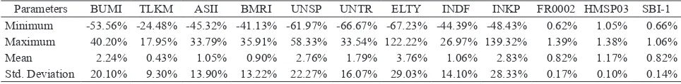
Statistical parameters
The model needs the statistical parameters
calculated from the defined historical data such as maximum value, minimum value, mean or average, and standard deviation. By using for-mulas and expressions as defined in previous chapter, it can be managed to provide the
num-bers as shown in Table 4.
Coefficient of correlation and covariance
After the standard deviation of the historical
data for each asset is defined, the twelve assets can be displayed in terms of their correlation and covariance in one table respectively. As previously described in formula expressions, the covariance, coefficient of correlation and
standard deviation are all parameters in single
formula. Covariance is actually the multiplica-tion of standard deviamultiplica-tions with its coefficient of correlation of the pair variables. It means, if the standard deviation of each assets are already known, the coefficient of correlation can be cal-culated, then covariance can be derived by
us-ing those both parameters.
Scenarios of weighting
There are about 17 possible weighting struc-tures which investors need to select. Each of Table 4. Statistical parameters
Parameters BUMI TLKM ASII BMRI UNSP UNTR ELTY INDF INKP FR0002 HMSP03 SBI-1
Minimum -53.56% -24.48% -45.32% -41.13% -61.97% -66.67% -67.23% -44.39% -48.43% 0.62% 1.05% 0.66%
Maximum 40.20% 17.95% 33.79% 35.91% 58.33% 33.54% 122.22% 26.97% 139.32% 1.39% 1.38% 1.06%
Mean 2.24% 0.43% 1.05% 0.90% 2.76% 1.79% 3.76% 1.06% 2.83% 0.82% 1.17% 0.82%
Std. Deviation 20.10% 9.30% 13.90% 13.22% 22.27% 16.07% 29.03% 14.10% 28.33% 0.17% 0.10% 0.14%
Table 5. Coefficient of correlations
Assets BUMI TLKM ASII BMRI UNSP UNTR ELTY INDF INKP FR0002 HMSP03 SBI-1
BUMI 1.000000 0.090074 0.411605 0.226659 0.500697 0.336622 0.356743 0.615977 0.289736 -0.686909 -0.500880 -0.403033
TLKM 0.090074 1.000000 0.615837 0.747954 0.170317 0.503846 0.102783 0.352198 -0.028306 -0.238225 -0.387428 0.137386
ASII 0.411605 0.615837 1.000000 0.716694 0.392185 0.696529 0.340343 0.617895 0.281944 -0.467562 -0.347023 -0.064465 BMRI 0.226659 0.747954 0.716694 1.000000 0.263234 0.584444 0.212763 0.478866 0.211777 -0.384160 -0.487087 0.015605 UNSP 0.500697 0.170317 0.392185 0.263234 1.000000 0.536381 0.749788 0.511952 0.451631 -0.236570 -0.255489 0.217558 UNTR 0.336622 0.503846 0.696529 0.584444 0.536381 1.000000 0.248696 0.698606 0.370941 -0.425010 -0.375439 -0.035726
ELTY 0.356743 0.102783 0.340343 0.212763 0.749788 0.248696 1.000000 0.297063 0.384324 -0.256742 -0.143943 0.095333
INDF 0.615977 0.352198 0.617895 0.478866 0.511952 0.698606 0.297063 1.000000 0.433811 -0.491270 -0.477787 -0.079515
those weighting structures yet still in verbal description of the investor. They need to be quantified in terms of value respectively. By us-ing Excel-based tool called Solver, the figures can be provided even to each asset as defined previously. This is the part where the risk mini-mization takes place for each of the weighting
structure.
Risks minimization
Stocks comprise nine selected assets, bonds comprise two (government and corporate bond), and SBI 1-month represents cash. Each of the weighting structure (17 possible structures) will have different share or portion for each 12 as-set. Solver found the weightings by conducting risk minimization to all weighting structures. Table 8 is the result of risk minimization pro-cess done by solver with 32,767 times of trials (repetitions).
It can be seen that each weighting structure has its own lowest risk in particular. That is be -cause each of them has its own variance and
standard deviation of portfolio as already de-fined. All those figures have yet nothing to do
with the rate of expected return since it will be done in separate process prior to the simulation.
Table 8 can be displayed together with the
ver-bal explanation of each weighting structure as
Table 9 shows. The structure number 16 has the
lowest risk weighting amongst all. The method
of obtaining the lowest risk is by utilizing solv-er of Excel add-ins.
Random number generation
Random numbers are generated to forecast the possible value occurred in the future for
each asset in the portfolio. They are defined by using uniform distribution for about 10,000 fig-ures, represents the large number of repetitions
Table 6. Covariance
Assets BUMI TLKM ASII BMRI UNSP UNTR ELTY INDF INKP FR0002 HMSP03 SBI-1
BUMI 0.040389 0.001684 0.011499 0.006024 0.022413 0.010873 0.020810 0.017459 0.016494 -0.000239 -0.000102 -0.000116
TLKM 0.001684 0.008655 0.007964 0.009202 0.003529 0.007534 0.002776 0.004621 -0.000746 -0.000038 -0.000036 0.000018
ASII 0.011499 0.007964 0.019324 0.013175 0.012143 0.015562 0.013733 0.012114 0.011102 -0.000112 -0.000049 -0.000013 BMRI 0.006024 0.009202 0.013175 0.017489 0.007754 0.012423 0.008167 0.008932 0.007933 -0.000088 -0.000065 0.000003 UNSP 0.022413 0.003529 0.012143 0.007754 0.049611 0.019202 0.048475 0.016082 0.028495 -0.000091 -0.000058 0.000069 UNTR 0.010873 0.007534 0.015562 0.012423 0.019202 0.025833 0.011602 0.015836 0.016888 -0.000118 -0.000061 -0.000008
ELTY 0.020810 0.002776 0.013733 0.008167 0.048475 0.011602 0.084253 0.012161 0.031600 -0.000129 -0.000042 0.000040
INDF 0.017459 0.004621 0.012114 0.008932 0.016082 0.015836 0.012161 0.019891 0.017331 -0.000120 -0.000068 -0.000016
INKP 0.016494 -0.000746 0.011102 0.007933 0.028495 0.016888 0.031600 0.017331 0.080240 -0.000060 0.000003 -0.000051 FR0002 -0.000239 -0.000038 -0.000112 -0.000088 -0.000091 -0.000118 -0.000129 -0.000120 -0.000060 0.000003 0.000001 0.000002 HMSP03 -0.000102 -0.000036 -0.000049 -0.000065 -0.000058 -0.000061 -0.000042 -0.000068 0.000003 0.000001 0.000001 0.000000 SBI-1 -0.000116 0.000018 -0.000013 0.000003 0.000069 -0.000008 0.000040 -0.000016 -0.000051 0.000002 0.000000 0.000002
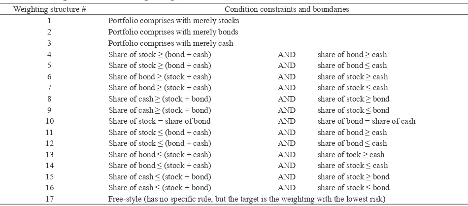
Table 7. The possible 17 weighting structures
Weighting structure # Condition constraints and boundaries
1 Portfolio comprises with merely stocks
2 Portfolio comprises with merely bonds
3 Portfolio comprises with merely cash
4 Share of stock ≥ (bond + cash) AND share of bond ≥ cash
5 Share of stock ≥ (bond + cash) AND share of bond ≤ cash
6 Share of bond ≥ (stock + cash) AND share of stock ≥ cash
7 Share of bond ≥ (stock + cash) AND share of stock ≤ cash
8 Share of cash ≥ (stock + bond) AND share of stock ≥ bond
9 Share of cash ≥ (stock + bond) AND share of stock ≤ bond
10 Share of stock = share of bond AND share of bond = share of cash
11 Share of stock ≤ (bond + cash) AND share of bond ≥ cash
12 Share of stock ≤ (bond + cash) AND share of bond ≤ cash 13 Share of bond ≤ (stock + cash) AND share of tock ≥ cash 14 Share of bond ≤ (stock + cash) AND share of stock ≤ cash
15 Share of cash ≤ (stock + bond) AND share of stock ≥ bond
16 Share of cash ≤ (stock + bond) AND share of stock ≤ bond
in order to have the high level of confidence or
low level of error in terms of statistics.
Expected return of portfolio
The expected return of portfolio can be de -rived from the multiplication of the weighting structure and the expected return of each asset.
The weighting structures have already been defined through risk minimization process and the expected returns of each asset have already been generated by random number generation in previous part. So the data has already
com-pleted in order to move on to the process of simulation.
Monte Carlo basic simulation
The basic simulation of Monte Carlo is actu-ally done through 10,000 times of repetitions according to the large numbers generated by
random function within uniform distribution.
These massive repetitions are done respectively to each weighting structures as previously de-fined. The results of the repetitions should pro-vide the model with all the statistical figures of each weighting structures, in this case the mean, standard deviation, minimum and
maxi-mum returns possible calculated and simulated.
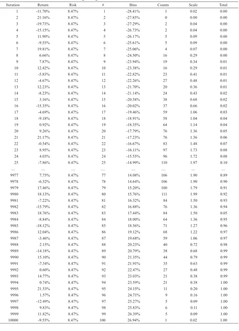
As can be seen from Table 10, the 10,000
massive iterations which represent the possible
expected returns on portfolio can be displayed
Table 8. The lowest risks for each weighting structures
Weight BUMI TLKM ASII BMRI UNSP UNTR ELTY INDF INKP FR0002 HMSP03 SBI-1 Stock Bond Cash Risk 1 10.58% 80.28% 0.00% 0.00% 0.00% 0.00% 0.38% 1.79% 6.97% 0.00% 0.00% 0.00% 100.00% 0.00% 0.00% 8.47%
2 0.00% 0.00% 0.00% 0.00% 0.00% 0.00% 0.00% 0.00% 0.00% 7.80% 92.20% 0.00% 0.00% 100.00% 0.00% 0.10%
3 0.00% 0.00% 0.00% 0.00% 0.00% 0.00% 0.00% 0.00% 0.00% 0.00% 0.00% 100.00% 0.00% 0.00% 100.00% 0.14% 4 5.53% 39.92% 0.00% 0.00% 0.00% 0.00% 0.19% 0.93% 3.43% 50.00% 0.00% 0.00% 50.00% 50.00% 0.00% 4.20%
5 5.53% 40.02% 0.00% 0.00% 0.00% 0.00% 0.15% 0.82% 3.48% 25.00% 0.00% 25.00% 50.00% 25.00% 25.00% 4.21% 6 0.30% 0.10% 0.00% 0.23% 0.00% 0.03% 0.00% 0.00% 0.00% 27.85% 70.83% 0.66% 0.66% 98.68% 0.66% 0.07% 7 0.24% 0.00% 0.00% 0.17% 0.00% 0.00% 0.00% 0.00% 0.00% 0.00% 67.84% 31.76% 0.41% 67.84% 31.76% 0.06% 8 0.29% 0.00% 0.00% 0.00% 0.00% 0.00% 0.00% 0.00% 0.01% 0.00% 0.30% 99.40% 0.30% 0.30% 99.40% 0.13% 9 0.26% 0.00% 0.00% 0.09% 0.00% 0.00% 0.00% 0.00% 0.00% 0.00% 49.65% 50.00% 0.35% 49.65% 50.00% 0.07% 10 3.83% 26.58% 0.00% 0.00% 0.00% 0.00% 0.08% 0.53% 2.31% 33.33% 0.00% 33.33% 33.33% 33.33% 33.33% 2.80%
11 0.24% 0.00% 0.00% 0.17% 0.00% 0.00% 0.00% 0.00% 0.00% 0.00% 69.38% 30.21% 0.41% 69.38% 30.21% 0.06%
12 0.26% 0.00% 0.00% 0.09% 0.00% 0.00% 0.00% 0.00% 0.00% 0.00% 49.83% 49.83% 0.35% 49.83% 49.83% 0.07%
13 2.99% 19.82% 0.00% 0.00% 0.00% 0.00% 0.06% 0.42% 1.70% 50.00% 0.00% 25.00% 25.00% 50.00% 25.00% 2.08% 14 0.26% 0.00% 0.00% 0.09% 0.00% 0.00% 0.00% 0.00% 0.00% 0.00% 50.00% 49.65% 0.35% 50.00% 49.65% 0.07%
15 2.88% 19.89% 0.00% 0.00% 0.00% 0.00% 0.00% 0.48% 1.75% 0.00% 25.00% 50.00% 25.00% 25.00% 50.00% 2.10% 16 0.24% 0.00% 0.00% 0.17% 0.00% 0.00% 0.00% 0.00% 0.00% 0.00% 69.19% 30.40% 0.41% 69.19% 30.40% 0.06% 17 0.24% 0.00% 0.00% 0.17% 0.00% 0.00% 0.00% 0.00% 0.00% 0.00% 69.08% 30.51% 0.41% 69.08% 30.51% 0.06%
Table 9. Conditional constraints and lowest risk WS
Weighting structure Conditional constraints and boundaries Stock Bond Cash Lowest risk
1 Portfolio comprises with merely stocks 100.00% 0.00% 0.00% 8.47%
2 Portfolio comprises with merely bonds 0.00% 100.00% 0.00% 0.10%
3 Portfolio comprises with merely cash 0.00% 0.00% 100.00% 0.14% 4 Share of stock ≥ (bond + cash) AND share of bond ≥ cash 50.00% 50.00% 0.00% 4.20%
5 Share of stock ≥ (bond + cash) AND share of bond ≤ cash 50.00% 25.00% 25.00% 4.21%
6 Share of bond ≥ (stock + cash) AND share of stock ≥ cash 0.66% 98.68% 0.66% 0.07%
7 Share of bond ≥ (stock + cash) AND share of stock ≤ cash 0.41% 67.84% 31.76% 0.06%
8 Share of cash ≥ (stock + bond) AND share of stock ≥ bond 0.30% 0.30% 99.40% 0.13%
9 Share of cash ≥ (stock + bond) AND share of stock ≤ bond 0.35% 49.65% 50.00% 0.07%
10 Share of stock = share of bond AND share of bond = share of cash 33.33% 33.33% 33.33% 2.80%
11 Share of stock ≤ (bond + cash) AND share of bond ≥ cash 0.41% 69.38% 30.21% 0.06%
12 Share of stock ≤ (bond + cash) AND share of bond ≤ cash 0.35% 49.83% 49.83% 0.07% 13 Share of bond ≤ (stock + cash) AND share of stock ≥ cash 25.00% 50.00% 25.00% 2.08% 14 Share of bond ≤ (stock + cash) AND share of stock ≤ cash 0.35% 50.00% 49.65% 0.07%
15 Share of cash ≤ (stock + bond) AND share of stock ≥ bond 25.00% 25.00% 50.00% 2.10%
16 Share of cash ≤ (stock + bond) AND share of stock ≤ bond 0.41% 69.19% 30.40% 0.06%
Table 10. Simulation result: Weighting structure 1
Iteration Return Risk # Bins Counts Scale Total
1 -11.70% 8.47% 1 -28.41% 1 0.02 0.00
2 21.16% 8.47% 2 -27.85% 0 0.00 0.00
3 -19.73% 8.47% 3 -27.29% 2 0.04 0.00
4 -15.15% 8.47% 4 -26.73% 2 0.04 0.00
5 11.90% 8.47% 5 -26.17% 5 0.09 0.00
6 -9.55% 8.47% 6 -25.61% 5 0.09 0.00
7 19.81% 8.47% 7 -25.06% 4 0.07 0.00
8 6.66% 8.47% 8 -24.50% 16 0.29 0.00
9 7.87% 8.47% 9 -23.94% 19 0.34 0.01
10 12.42% 8.47% 10 -23.38% 16 0.29 0.01
11 -5.83% 8.47% 11 -22.82% 23 0.41 0.01
12 -4.67% 8.47% 12 -22.26% 27 0.48 0.01
13 12.23% 8.47% 13 -21.70% 20 0.36 0.01
14 -8.23% 8.47% 14 -21.14% 24 0.43 0.02
15 3.16% 8.47% 15 -20.58% 38 0.68 0.02
16 -15.35% 8.47% 16 -20.02% 37 0.66 0.02
17 -4.69% 8.47% 17 -19.46% 59 1.06 0.03
18 -9.18% 8.47% 18 -18.91% 58 1.04 0.04
19 0.92% 8.47% 19 -18.35% 64 1.14 0.04
20 9.26% 8.47% 20 -17.79% 76 1.36 0.05
21 21.17% 8.47% 21 -17.23% 76 1.36 0.06
22 -0.54% 8.47% 22 -16.67% 83 1.48 0.07
23 8.95% 8.47% 23 -16.11% 97 1.73 0.08
24 4.03% 8.47% 24 -15.55% 96 1.72 0.08
25 -7.86% 8.47% 25 -14.99% 110 1.97 0.10
… … … …
9977 7.75% 8.47% 77 14.08% 106 1.90 0.89
9978 -6.32% 8.47% 78 14.64% 106 1.90 0.90
9979 17.46% 8.47% 79 15.20% 100 1.79 0.91
9980 18.13% 8.47% 80 15.76% 111 1.99 0.92
9981 -7.22% 8.47% 81 16.32% 84 1.50 0.93
9982 -15.79% 8.47% 82 16.88% 76 1.36 0.94
9983 18.76% 8.47% 83 17.44% 84 1.50 0.05
9984 -8.84% 8.47% 84 18.00% 64 1.36 0.95
9985 -18.12% 8.47% 85 18.56% 71 1.27 0.96
9986 12.04% 8.47% 86 19.12% 68 1.22 0.97
9987 -3.46% 8.47% 87 19.68% 59 1.06 0.97
9988 2.15% 8.47% 88 20.23% 40 0.72 0.98
9989 -14.18% 8.47% 89 20.79% 38 0.68 0.99
9990 15.10% 8.47% 90 21.35% 44 0.79 0.99
9991 -7.34% 8.47% 91 21.91% 35 0.63 0.99
9992 0.60% 8.47% 92 22.47% 27 0.48 0.99
9993 14.77% 8.47% 93 23.03% 21 0.38 0.99
9994 0.74% 8.47% 94 23.59% 21 0.38 1.00
9995 21.53% 8.47% 95 24.15% 11 0.20 1.00
9996 1.57% 8.47% 96 24.71% 9 0.16 1.00
9997 -12.49% 8.47% 97 25.27% 5 0.09 1.00
9998 9.83% 8.47% 98 25.83% 6 0.11 1.00
9999 11.82% 8.47% 99 26.39% 5 0.09 1.00
10000 -9.55% 8.47% 100 26.94% 1 0.02 1.00
Statistical summary
Minimum Maximum Median Mean Std. deviation Probability UCL LCL
in a simple statistical view. That view will show
the investor regarding the probability of the ex-pected rate of return of the portfolio may fall
with such weighting structure. The view of the
statistical result can be seen as Figure 7. The absis represents the bins, which is the range
dis-tribution of expected rate of returns of weight -ing structure 1 portfolio. The minimum return is
around -28% and the maximum return is around 27%. The ordinate represents the count or fre-quency of certain bin occurred. At glance see, the pattern is kind of normal distribution, which
has some level of skewness and kurtosis. Below are the WS1 statistical measurement which also
will be presented by other weighting structures (the other 16 weighting structures).
• Maximum = 26.94%
• Minimum = -28.41%
• Mean = -0.18%
• Standard deviation = 11.01%
By using the statistical routine function of the Excel (percentrank), the probability of some
level of target return can be calculated with this weighting structure. It was stated that the target
return of the investor is about 1.5% per month net. Therefore, the calculation of the probabil-ity has come to the level of 45% chance to get
the level of that target return.
Optimal result determination
After the simulations are done to the rest of
the weighting structures, then there should be about 17 outcomes of simulation which are go-ing to be selected, regardgo-ing the one that will be
the best options of all weighting structures. The
complete process of optimization and simula-tions may provide investor with this table sum-mary as shown in the next table.
The lowest risk of portfolio has already been determined, it is the weighting structure 16.
But that was historical. In terms of forecast
-ing by us-ing the simulation, the lowest volatil-ity of portfolio return is actually derived by the weighting structure 2 eventually. This will be emphasized more in the efficient frontier
plot-ting part later.
As can be seen, that the first weighting
struc-ture resulted with the highest return possible but also with the highest risk although the prob
-ability of gaining the target return is still there, about 45% chance to achieve 1.5% target re-turn per month. For rational investor, especial-ly for risk-averse kind of investor, this can be very risky. The lowest risk resulted by the sec-ond weighting structure with bsec-ond-dominated portfolio. Although the probability of earning
1.5% target return were out of range (since the minimum is only about 1.02% and maximum is about 1.38%), but with mean average of return about 1.25%, particularly for risk-averse type of investor, this is a kind of best portfolio that
investor can earn.
Therefore, the selection of portfolio will fall
to the second weighting structure where the pro
-portion is 0% in stocks, 0% in cash, but 7.8% in FR00002 and 92.20% in HMSP03. Based on the last three years of historical asset’s data,
then its better to allocate the entire fund in sec
-ond weighting structure. In terms of probability and statistics, this weighting structure will
pro-vide investor with lowest standard deviation of portfolio return.
Efficient frontier plotting
Once expected returns, standard deviation and correlation coefficients have been deter-mined, then the list of “optimal” portfolios can
be created. These portfolios lie on a graph line
called the “efficient frontier,” which represents
the asset mix with the highest expected returns
for each given level of risk. By plotting every
portfolio representing a given level of risk and
expected return, it can be able to trace a line connecting all the efficient portfolios, all these dots usually known as locus. This line forms the efficient frontier. Rational investors limit the selection in the efficient frontier and to the specific portfolio that represents their own risk
Table 12. Risk, return, and Sharpe ratios of each WS
WEIGHTING STRUCTURES CONDITIONAL CONSTRAINTS RISK RETURN SHARPE
1 Portfolio comprises all stocks 8.47 % 0.81 % 0.0049
2 Portfolio comprises all bonds 0.10 % 1.14% 3.7128
3 Portfolio comprises all cash 0.14 % 0.82 % 0.3618
4 Share of stock ≥ (bond+cash) AND share of bond ≥ cash 4.20 % 0.82 % 0.0117
5 Share of stock ≥ (bond+cash) AND share of bond ≤ cash 4.21 % 0.82 % 0.0115
6 Share of bond ≥ (stock+cash) AND share of stock ≥ cash 0.07 % 1.07 % 4.5195
7 Share of bond ≥ (stock+cash) AND share of stock ≤ cash 0.06 % 1.06 % 4.9088
8 Share of cash ≥ (stock+bond) AND share of stock ≥ bond 0.13 % 0.83 % 0.4390
9 Share of cash ≥ (stock+bond) AND share of stock ≤ bond 0.07 % 1.00 % 3.3720
10 Share of stock = bond = cash 2.80 % 0.82 % 0.0182
11 Share of stock ≤ (bond+cash) AND share of bond ≥ cash 0.06 % 1.07 % 5.0023
12 Share of stock ≤ (bond+cash) AND share of bond ≤ cash 0.07 % 1.00 % 3.3879
13 Share of bond ≤ (stock+cash) AND share of stock ≥ cash 2.08 % 0.82 % 0.0251
14 Share of bond ≤ (stock+cash) AND share of stock ≤ cash 0.07 % 1.00 % 3.4039
15 Share of cash ≤ (stock+bond) AND share of stock ≥ bond 2.10 % 0.91 % 0.0655
16 Share of cash ≤ (stock+bond) AND share of stock ≤ bond 0.06 % 1.07 % 4.9914
17 Free-style 0.06 % 1.07 % 4.9851
Table 11. Weighting structures simulation result
Wgt Portfolio Weight Structures Min Max Mean Stdev Pr(Return ≥ 1.5%) Remarks
1 All stocks -28.41 % 26.94 % -0.18 % 11.01 % 45.10 % Highest probability, highest return and risk
2 All bonds 1.02 % 1.38 % 1.20 % 0.09 % out of range Highest possible return, the lowest risk
3 All cash 0.66 % 1.06 % 0.86 % 0.12 % out of range
4 Stock ≥ bond + cash and bond ≥ cash -13.66 % 13.97 % 0.38 % 0.34 % 43.40 %
5 Stock ≥ bond + cash and bond ≤ cash -13.81 % 14.11 % 0.36 % 0.31 % 43.40 % 6 Bond ≥ stock + cash and stock ≥ cash 0.69 % 1.51 % 1.12 % 1.12 % 0.10 % 7 Bond ≥ stock + cash and stock ≤ cash 0.77 % 1.41 % 1.08 % 1.08 % out of range
8 Cash ≥ stock + bond and stock ≥ bond 0.51 % 1.19 % 0.85 % 0.85 % out of range
9 Cash ≥ stock + bond and stock ≤ bond 0.71 % 1.33 % 1.02 % 1.02 % out of range
10 Stock = bond = cash -8.93 % 9.79 % 0.54 % 0.51 % 41.60 %
11 Stock ≤ bond + cash and bond ≥ cash 0.77 % 1.42 % 1.09 % 1.09 % out of range the highest Sharpe prior to simulation
12 Stock ≤ bond + cash and bond ≤ cash 0.71 % 1.33 % 1.02 % 1.02 % out of range 13 Bond ≤ stock + cash and stock ≥ cash -6.43 % 7.58 % 0.63 % 0.63 % 39.80 % 14 Bond ≤ stock + cash and stock ≤ cash 0.71 % 1.33 % 1.02 % 1.02 % out of range
15 Cash ≤ stock + bond and stock ≥ bond -6.62 % 7.61 % 0.65 % 0.65 % 40.10 %
16 Cash ≤ stock + bond and stock ≤ bond 0.77 % 1.42 % 1.09 % 1.09 % out of range the lowest risk prior to simulation
tolerance level. Therefore, the other way to find out the optimal portfolios is by utilizing
effi-cient frontier using parameters of the portfolio
selected. As shown by the table before, the low-est risk amongst the structures is about 0.0593% and this figure can be plotted in the area of
effi-cient frontier in the investment quadrant. Figure
8 represents the efficient frontier of the optimal
portfolios.
As shown in Figure 8, the efficient frontier can be used to find out the lowest risk
portfo-lio and the best one amongst all of then (tan
-gency portfolio should be located in right side). Referring to the graph in Figure 8, the rational
investor can pinpoint a single portfolio weight
-ing (within the area of efficient frontier) which is actually better than other optimal portfolios from some point of view (return, risk, or Sharpe ratio).
Anyway, this is the current view by using historical data of the portfolio. The objective as initially defined in this research is to find
out the single weighting structure amongst all
structured weightings with lowest volatility of its portfolio return or mean. By combining the modern portfolio theory with solver and basic Monte Carlo for simulating the future event,
the weighting structure with the lowest stand
-ard deviation of portfolio mean can be possibly
obtained.
By only depending on historical view, the investor may finally misled selecting the
port-folio with the highest Sharpe ratio weighting
structure or the lowest risk one, or even the highest return. By fully utilize the simulation of random data which will be probably occured in the future events (in terms of probability using uniform distribution), the decision might end up differently for the investors. As shown by Table 12, the weighting structure with highest Sharpe ratio is located in the tangency portfolio (WS-11 at Table 12), but the structure with the lowest risk is shown by WS-16.
(WS-11 at Table 12), but the structure with the lowest risk is shown by WS-16. From his-torical point of view, choice of portfolios may fall to the WS-11 and WS-16. Nevertheless, us-ing the simulation to forecast the future events,
the weighting structure with lowest standard
deviation of its portfolio mean is eventually the WS-2.
Conclusion
The research has come to a certain conclu -sions based on the three issues which mentioned
in the very beginning part of this article. As the result has shown, stocks can be allocated much
in a portfolio of investment but it should be done
in a way that do not harm or jeopardize the port-folio as whole in terms of its risk or volatility. After assessing the high volatility of some asset
classes which had been pooled together within
an investment portfolio, it surely does not very
wise for investors to keep the portfolio weight -ing in dominant stock instead of dominant bond
or cash. By making the decision to switch the portfolio into much more in bond or cash, the risk of portfolio can be significantly reduced
but also in the same time limiting the potential return of portfolio that can be earned. As for the
risk-averse type of investor, the dominant bond and cash may be more preferred.
As the portfolio should be dominated by the fixed income instrument, then the next issue will be the share figure for each one of them. Based on the calculation done in this research,
the best structured weighting should be the
number two (WS-2) since it can provide
inves-tors with lowest risk of its forecasted mean re
-turn. The choice of portfolio comprises 0% in stocks, 0% in cash, but 7.8% in FR00002 and 92.20% in HMSP03.
The world market is now in recession and
people are currently living in it. Prior to the recession, investors are all enjoying the great earnings they have got from trading stocks and
other high risk instruments when market is in
bullish trend. Therefore, if it merely based on the historical figure or nothing to do with the forecasting figures of the returns, then investors
should have different choices of best portfolio.
Based on the risk minimization process, the
investor should be selecting the one with the greatest Sharpe ratio of all structured weight
-ings, that is the 11th WS. It comprises 0.41%
stocks, 69.38% bonds and 30.21% cash. The
portfolio risk of this choice of portfolio is the lowest among them all but with the highest lev -el of Sharpe ratio.
References
Barron’s Educational Series (1991), Dictionary of Finance and Investment Terms, 3rd Ed.
Baumohl, B. (2008), The Secrets of Economic Indicators: Hidden Clues to Future Eco-nomic Trends and Investment Opportunities 2ndEd., Wharton School Publishing.
Bodie, Z., Kane, A., and Marcus, A.J. (2008),
Investments 7th Ed., New York:
McGraw-Hill.
Cooper, R. (2004), Corporate Treasury and Cash Management, New York: Palgrave MacMillan.
Damodaran, A. (2002), Investment Valuation: Tools and Techniques for Determining the Value of Any Asset 2nd Edition, New York:
John Wiley & Sons.
Dupire, B. (1998), Monte Carlo: Methodolo-gies and Application for Pricing and Risk Management, Risk Books.
Fabozzi, F.J. (1999), Investment Management 2nd Ed., Upper Saddle River: Prentice-Hall,
Inc.
Fischer, D.E. and Jordan, R.J. (1991), Security Analysis and Portfolio Management 5th Ed.,
Upper Saddle River: Prentice-Hall, Inc. Foldvary, F.E. (2007), The Depression of 2008,
Portable Document Format: The Gutenberg
Press.
Gibson, R.C. (1996), Asset Allocation: Balanc-ing Financial Risk 2nd Ed., Times Mirror:
Higher Education Group.
Kritzman, M.P. (1990), Asset Allocation for In-stitutional Portfolios, Business One Irwin.
Levin, R.I. and Rubin, D.S. (1998), Statistics for Management 7th Ed., New Jersey:
Pren-tice-Hall, Inc.
Markowitz, H. (1952), Portfolio Selection,
Journal of Finance, 7(1), 77-91.
McDonnell, P.J. (2008), Optimal Portfolio Modeling, New Jersey: John Wiley & Sons, Inc.
McLeish, D.L. (2004), Monte Carlo Simulation and Finance, eBook Edition: New Jersey:
John Wiley & Sons, Inc.
Papp, J.N. (1991), Portfolio Results Enhanced--Using Markowitz Increases Returns without Added Risk, Pension & Investments.
Richard, B.A., Stewart, M.C., and Franklin, A. (2008), Principles of Corporate Finance 9th
Ed., New York: McGraw-Hill.
Savage, S. (2009), The Flaw of Averages: Why We Underestimate Risk in the Face of Un-certainty, New Jersey: John Wiley & Sons, Inc.
River: Pearson Prentice Hall.
Vince, R. (1990), Portfolio Management For-mulas: Mathematical Trading Methods for the Futures, Options, and Stock Markets,
New Jersey: John Wiley & Sons.
Williams, J.B. (1997), The Theory of Invest-ment Value, Amsterdam: North-Holland