7KHUHWXUQVWRHGXFDWLRQLQ,QGRQHVLD3RVWUHIRUPHVWLPDWHV
/RVLQD3XUQDVWXWL5XKXO6DOLP0RKDPPDG$EGXO0XQLP-RDUGHUThe Journal of Developing Areas, Volume 49, Number 3, Summer
2015, pp. 183-204 (Article)
3XEOLVKHGE\7HQQHVVHH6WDWH8QLYHUVLW\&ROOHJHRI%XVLQHVV
For additional information about this article
T h e J o u r n a l o f D e v e l o p i n g A r e a s
Volume 49 No. 3 Summer 2015THE RETURNS TO EDUCATION IN
INDONESIA: POST REFORM ESTIMATES
Losina Purnastuti
Yogyakarta State University, Indonesia
Ruhul Salim
Mohammad Abdul Munim Joarder
Curtin University, Australia
ABSTRACT
The profitability of an investment in education in Indonesia has been a discussed issue for the past decades. Both Deolalikar (1993) and Duflo (2001) provided comprehensive estimates of returns to investment in education in Indonesia and both of them argued that schooling was a profitable investment. This paper updates the evidence on the profitability of an investment in education in Indonesia, using OLS and IV approaches. It describes the statistical relationship among market earnings, years of schooling, age and job tenure (experience), and quadratics of age and tenure, marital status, male-female and rural-urban dummies. In the analysis, we use primary data from the Indonesian Family Life Survey 4 (IFLS4). IFLS4 is a nationally representative sample comprising 13,536 households and 50,580 individuals, spread across provinces on the islands of Java, Sumatra, Bali, West Nusa Tenggara, Kalimantan, and Sulawesi. The earnings function is estimated on three samples: a combined sample of males and females (with a female intercept shift term), and separate samples of male and female workers. The empirical results show that the returns to schooling in Indonesia are 4.72 per cent for the combined sample, 4.36 per cent for males, and 5.26 per cent for females. However, the relationship between years of schooling and earnings is not statistically significant in any of the IV estimations. We also make comparisons with the findings of Duflo (2001), based on earlier data for 1995. These comparisons enable an assessment of any changes in the ability bias over this period of market reform. The IV estimates are the same as, or greater than, the OLS estimates. This is consistent with the literature for developed countries, and suggests that ability does not attract a wage premium but may be correlated with the instruments. Although adopting the IV approach increases the estimated returns to schooling in Indonesia, these returns remain low compared to other Asian as well as less developed countries. Therefore, the market-oriented economic reforms that has been going on over the past several decades should be evaluated by the policy makers considering whether these reforms generating higher jobless growth or not and take proper policy measure, if there is any.
JEL Classifications:I21, I22, J30, J31
Keywords: Earnings, Experience, Returns to Schooling, Instrumental Variable Corresponding Author’s Email Address: [email protected]
INTRODUCTION
184
system initiated in Australia, and now used more widely, such as in Thailand and Ethiopia (Chapman, 1997). It has been argued that part of the magnitude quantified as a return to schooling in many countries is in fact an omitted variable (ability) bias, though it has also been shown that the upward bias to the true return to schooling from this source is offset by measurement error (Ashenfelter and Krueger, 1994). Similar themes are found in research into the determinants of earnings in developing countries. In Indonesia, studies by Deolalikar (1993) and Duflo (2001) have established that schooling is a profitable investment. Duflo reported, however, that based on analyses of data collected in 1995, the IV estimates of the return to schooling were broadly the same as the OLS estimates. This suggests that the upward ability bias was either relatively small, or offset by downward measurement error bias, as in Western labour markets.
Over the past three decades, Indonesia has embarked on an ambitious program of market-oriented economic reforms. The early phases of this, during the Suharto era, were driven first by the oil boom, and then by deregulation. After the Suharto era the market-oriented economic reforms in Indonesia were basically imposed by the IMF (Kalinowski, 2007). These changes were associated with a considerable shift in employment away from the agricultural sector towards manufacturing, transportation, storage, and communication, and the community, social and personal services industries. Thus, agriculture’s employment share declined from 56.30 percent in 1980 to 39.87 percent by 2010. Market reforms are often expected to lead to a greater alignment of wages with productivity-related characteristics. This is what has occurred in China (Zhang et al. 2005). In this situation, it would be expected that the true return to schooling would have increased and the ability bias widened. Therefore, the estimation of the return to schooling in the contemporary Indonesian labour market should produce results different from those reported by Duflo (2001). In this article we investigate the return to schooling in Indonesia, using both OLS and IV methods, and data for 2007-2008. Comparison of the results from these more contemporary data with Duflo’s (2001) findings, based on the earlier data for 1995, enable us to make an assessment of changes in the true return to schooling and in the ability bias over this period of market reform.
The rest of the article is structured as follows. A conceptual framework is presented in Section 2, followed by a brief review of the literature in Section 3. Section 4 outlines the data set that provides the basis for the empirical analysis of the determinants of earnings in Indonesia. The OLS and IV results are presented and discussed in Section 5. Section 6 summarises the findings and concludes.
CONCEPTUAL FRAMEWORK
A worker’s earnings are influenced by a wide range of factors, including personal characteristics and labour market experience. However, in the exposition that follows it is useful to consider only a simple process where earnings are a function of years of schooling (S) and the level of ability (A), namely
ln
Y
f S A
( , )
. The earnings-schooling relationship for a person of ability levelA
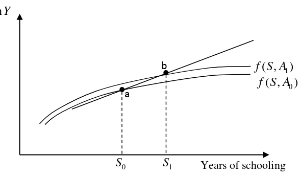
0 is depicted in the bottom profile in Figure 1.185
[image:4.612.180.475.276.447.2]argued that earnings determination places only a modest weight on productivity-related factors, such as schooling or ability, and more weight on other factors, such as nepotism. Accordingly, it is expected that in Indonesia in the early stages of market reform, the earnings-schooling profile
f S A
( ,
0)
in Figure 1 would be reasonably flat. However, it would be expected that the earnings-education profile for the more able will be above that for their less-able counterparts by only a small margin. This is depicted in the second curve in Figure 1, where the earnings profile for the more able person (A
1) lies above that for the less-able person (A
0), but only marginally.Figure 1: Hypothetical Earnings-Schooling Profile by Ability (Ability has a Limited Effect)
When estimating the return to schooling, in the absence of information on ability, researchers compare the earnings of individuals with schooling level
S
1 (point ‘b’ in the diagram) with the earnings of individuals with schooling levelS
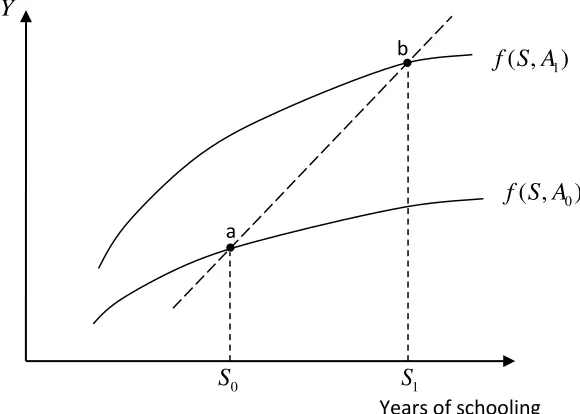
0 (point ‘a’ onthe diagram). This is given by the slope of the linear line through points ‘a’ and ‘b’. This slope will differ from the slope of the earnings-schooling profiles, but by only a minor amount in the current scenario. The difference between the slope of the linear line in Figure 1 and that of the earnings-schooling profile is the ability bias. The small ability bias in the estimated return to schooling apparent here is simply attributable to the minor role that ability plays in earnings determination. The pattern evident in many countries that embark on a program of market reform is that earnings become more aligned with productivity (Zhang et al. 2005; Ren and Miller, 2012). As a result, the earnings-schooling profile will steepen and we would have earnings-earnings-schooling profiles as depicted in Figure 2, where again ability level
A
1
A
0. It is apparent from Figure 2 that not only is the return to schooling (the slope of the curved earnings-schooling profile) greater than in Figure 1, but the ability bias (the difference between the slopes of the linear line through points ‘a’ and ‘b’ and the earnings-schooling profile) is also larger thanln
Y
b
1
( ,
)
f S A
0
( ,
)
f S A
a
1
S
0
186
previously. One response by researchers to the ability bias is to apply an instrumental variables (IV) estimator. The IV approach also accommodates classical measurement error in the schooling variable. With valid instruments, the instrumental variables estimator will give a consistent estimate of the return to schooling, which will be lower than the OLS estimate. In cases where the instruments are not strictly exogenous, due, for example, to correlation with the unobserved ability, the IV estimate of the return to schooling will be upward biased also (Card, 1999).1 Comparison of IV estimates with
[image:5.612.180.470.341.548.2]OLS estimates, under a number of different sets of instruments, can therefore inform on the importance of ability bias in the estimation of the return to schooling. From this perspective, the starting point for the assessment in this paper is the research by Duflo (2001), based on data collected in 1995. Duflo (2001) concluded that the IV estimates of the returns to schooling were not significantly different from the OLS estimates, which suggests that in 1995 the upward ability bias approximately offset the downward measurement error bias.
FIGURE 2: HYPOTHETICAL EARNINGS-SCHOOLING PROFILE BY ABILITY (ABILITY HAS A MORE MAJOR EFFECT)
LITERATURE REVIEW
There have been a good number of studies employing an IV approach for measuring returns to schooling for both developed and developing countries. Due to space limitation, some important recent studies from developing countries are reviewed here. Cheidvasser and Silva (2007) used a representative sample of the Russian Federation, the Russian Longitudinal Monitoring Survey, to estimate the return to education. The authors complemented their OLS results with IV estimates and showed that the exogeneity of the education variable could not be rejected. The returns to education estimated for Russia
Years of schooling
ln
Y
0
( ,
)
f S A
1
( ,
)
f S A
a
b
0
187
were quite low, ranging around 1-2.3 per cent for men and around 3.7-5.9 per cent for women.
Duflo (2001) examined the return to schooling in Indonesia using data from the 1995 inter-censal survey of Indonesia (SUPAS). She concentrated on adult males born between 1950 and 1972. A feature of this study was that individual-level data on education and wages were linked with district-level data on the number of new Sekolah Dasar (Primary Schools) INPRES built between 1973-1974 and 1978-1979 in the worker’s region of birth.2 The number of schools built in the individual’s region of birth
and the individual’s age when the program was launched was then used to determine the exposure of an individual to the program, and this provided the instruments for the wage equation. Duflo confirmed that these instruments have good explanatory power in the first-stage regression of her IV approach. The IV estimates of the returns to education ranged from 6.8 to 10.6 per cent, though these estimates were not significantly different from the OLS estimates. Based on this evidence Duflo (2001) concluded that OLS coefficients were not biased upwards.
Comola and Mello (2010) also examined the returns to schooling in the Indonesian labour market. They used data from the 2004 Indonesian labour market survey (Sakernas). The endogeneity of educational attainment problem was handled by instrumenting years of schooling by exposure to Sekolah Dasar INPRES, a similar identification strategy as Duflo (2001). The estimate of the return to education from a Mincerian wage equation for 2004 obtained by standard OLS ranged from 9.49 per cent to 10.32 per cent. The estimated coefficients were very similar whether or not educational attainment is treated as endogenous. This supports Duflo’s (2001) conclusion that OLS estimates are not likely to be biased upwards. Thus, both these studies report that there is little evidence of ability bias in the OLS estimates of the return to schooling in Indonesia. This issue is investigated further below, using more recent data, and a wider set of instruments.
DATA AND ESTIMATING EQUATION
The data set used in the empirical analysis is the Indonesian Family Life Survey 4 (IFLS4). IFLS4 is a nationally representative sample comprising 13,536 households and 50,580 individuals, spread across provinces on the islands of Java, Sumatra, Bali, West Nusa Tenggara, Kalimantan, and Sulawesi. Together these provinces encompass approximately 83 per cent of the Indonesian population and much of its heterogeneity. IFLS4 was fielded in late 2007 and early 2008. For this analysis of the returns to schooling, the sample is restricted to individuals 15 to 65 years old, who were not full-time students, reported non-missing labour market income, provided information on schooling, and supplied information on family background. Persons in the military during the survey week are omitted, as it is generally argued that the wages of those in the armed services do not necessary reflect market forces. A total of 4596 observations satisfy these criteria and are utilised in the analysis. The construction of the main variables is discussed below, and the definitions are given in Table 1.
188
t t t t t t t t t iurban
married
femde
tenure
tenure
age
age
yrsch
earnings
8 7 6 2 5 4 2 3 2 1 0)
ln(
(1) i t tZ
yrsch
(2)where earnings denotes monthly earnings, yrsch is the years of schooling for the worker, ageis age, which is our measure of general labour market experience, tenure represents job tenure, female is a dummy variable for gender, married is a dummy variable for marital status, and urban is a residential dummy (urban versus rural). Z is the vector of variables that are held to account for the variation in the years of
schooling.
It contains a constant term, all the exogenous variables from Equation (1), plus the identifying instruments. These are described below. The dependent variable in this analysis is the natural logarithm of monthly earnings. These monthly earnings include the value of all benefits secured by an individual in their job. The unit of measurement is rupiah (Rp) (US$1 was approximately equal to Rp9,000 at the time of the 2007/2008 survey). The two main explanatory variables are the years of schooling and age as a measure of years of general labour market experience. The years of schooling are compiled from the survey question on the highest level of qualification. Age is used as the measure of general labour market activity.TABLE 1: VARIABLE DEFINITIONS
Symbols Variables Definition
Ln (earnings) Monthly Earnings (log) Monthly earnings in log form.
Yrsch Years of schooling Number of years of schooling of the respondent.
Age Age Age of individual.
Age2 Age2 The square of age.
Tenure Tenure Work experience in the present job.
Tenure2 Tenure2 The squared of work experience in the present job. Female Dummy for gender 1 if individual is female; 0 otherwise.
Married Dummy for marital status 1 if individual is married; 0 otherwise. Urban Dummy for area 1 if individual lives in urban area; 0 otherwise. Father’s schooling Father’s years of schooling Number of years of schooling of the respondent’s
father.
Mother’s schooling Mother’s years of schooling Number of years of schooling of the respondent’s mother.
CSAL-1 Dummy for six year compulsory education
1 if individual was born in 1977 and later; 0 otherwise.
CSAL-2 Dummy for nine year compulsory education
1 if individual was born in 1987 and later; 0 otherwise.
INPRES Program Dummy for INRES program 1 if individual was born in 1967 and later; 0 otherwise.
Preschool Dummy for preschool 1 if individual attended preschool; 0 otherwise. Delayed PS The age of primary school
enrolment
Individual’s age when the first time enrol to primary school.
189
training and knowledge. The second variable is gender; a variable that distinguishes females from males is entered into the estimating equation to capture gender discrimination, and the earnings consequences of unobserved work-home duties-leisure outcomes that are correlated with gender. The third variable is marital status, which should have consequences for labour market earnings: positive for males and negative for females. The last variable is a residential dummy (rural versus urban), which is intended to control for the earnings differential between urban and rural areas.
The IFLS4 data base contains a number of potential instruments for the years of schooling variable. These can be viewed in terms of two broad categories. The first category comprises variables that are the same for all individuals in a given age category. We term these natural (or cohort) instruments. There are three of these variables, namely a dummy variable for the presidential instruction (INPRES) program, a dummy variable for the first compulsory school attendance law (CSAL-1), and a dummy variable for the second compulsory school attendance law (CSAL-2). The second category comprises variables that vary across individuals in a given age category. We term these individual instruments. Included here are father’s years of schooling, mother’s years of schooling, a dummy variable for preschool attendance, and a variable that records delayed enrolment in primary school (age of primary school enrolment).
190
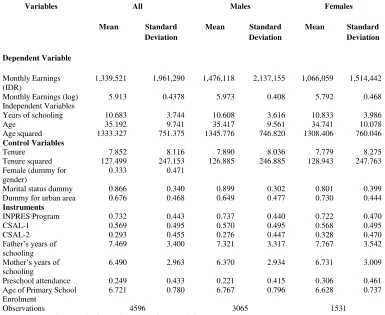
TABLE 2: SUMMARY STATISTICS
Variables All Males Females
Mean Standard Deviation
Mean Standard Deviation
Mean Standard Deviation
Dependent Variable
Monthly Earnings (IDR)
1,339,521 1,961,290 1,476,118 2,137,155 1,066,059 1,514,442
Monthly Earnings (log) 5.913 0.4378 5.973 0.408 5.792 0.468 Independent Variables
Years of schooling 10.683 3.744 10.608 3.616 10.833 3.986
Age 35.192 9.741 35.417 9.561 34.741 10.078
Agesquared 1333.327 751.375 1345.776 746.820 1308.406 760.046 Control Variables
Tenure 7.852 8.116 7.890 8.036 7.779 8.275
Tenure squared 127.499 247.153 126.885 246.885 128.943 247.763 Female (dummy for
gender)
0.333 0.471
Marital status dummy 0.866 0.340 0.899 0.302 0.801 0.399 Dummy for urban area 0.676 0.468 0.649 0.477 0.730 0.444 Instruments
INPRES Program 0.732 0.443 0.737 0.440 0.722 0.470
CSAL-1 0.569 0.495 0.570 0.495 0.568 0.495
CSAL-2 0.293 0.455 0.276 0.447 0.328 0.470
Father’s years of schooling
7.469 3.400 7.321 3.317 7.767 3.542
Mother’s years of schooling
6.490 2.963 6.370 2.934 6.731 3.009
Preschool attendance 0.249 0.433 0.221 0.415 0.306 0.461 Age of Primary School
Enrolment
6.721 0.780 6.767 0.796 6.628 0.737
Observations 4596 3065 1531
Source: Authors’ calculation based on the IFLS4 data set.
STATISTICAL ANALYSES
OLS Results
191
selection correction in analysis of the IFLS4 also showed that this was of limited consequence (Purnastuti, Miller and Salim, 2013).
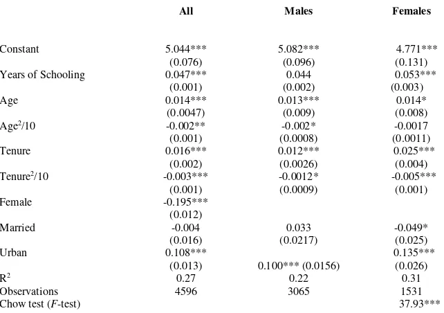
[image:10.612.139.460.393.619.2]The earnings function is estimated on three samples: a combined sample of males and females (with a female intercept shift term), and separate samples of male and female workers. The estimates of the return to schooling in Indonesia in Table 3 are 4.72 per cent for the combined sample, 4.36 per cent for males, and 5.26 per cent for females. The gender differential in the return to schooling is turn out to be statistically significant. This result is consistent with the findings of earlier empirical studies for Indonesia, such as Deolalikar (1993) and Behrman and Deolalikar (1993). These estimates of the return to schooling are substantially smaller than the Psacharopoulos (1981) average estimate of 14 per cent for Less Developed Countries, and the Psacharopoulos (1994) average estimate of 9.6 per cent for Asian countries. However, our results are in agreement with some empirical studies, for example: Jamison and Gaag (1987) for China, Flanagan (1998) for the Czech Republic, Aromolaran (2006) for Nigeria, and Aslam, Bari, and Kingdon (2012) for Pakistan. A relatively low rate of return to schooling in our study is due to several reasons. A likely candidate in this regard is a decline in the quality of schools and a significant increase in the supply of educated workers in the labour market, due to a combination of events such as the massive school construction program in 1973 and 1974 and the compulsory education program in 1984 that provides the basis for one of our sets of instruments.
TABLE 3: OLS ESTIMATES OF MINCERIAN EARNINGS FUNCTION
All Males Females
Constant 5.044***
(0.076)
5.082*** (0.096)
4.771*** (0.131) Years of Schooling 0.047***
(0.001)
0.044 (0.002)
0.053*** (0.003)
Age 0.014***
(0.0047)
0.013*** (0.009)
0.014* (0.008)
Age2/10 -0.002**
(0.001)
-0.002* (0.0008)
-0.0017 (0.0011)
Tenure 0.016***
(0.002)
0.012*** (0.0026)
0.025*** (0.004) Tenure2/10 -0.003***
(0.001)
-0.0012* (0.0009)
-0.005*** (0.001)
Female -0.195***
(0.012)
Married -0.004
(0.016)
0.033 (0.0217)
-0.049* (0.025)
Urban 0.108***
(0.013) 0.100*** (0.0156)
0.135*** (0.026)
R2 0.27 0.22 0.31
Observations 4596 3065 1531
Chow test (F-test) 37.93***
192
The coefficients on the age variable and its squared term have the expected signs, and portray the usual concavity of the age-earnings profile, although less so in the case of females than for males. Among labour market entrants (age = 16) the return on an extra year of labour market activity is 0.8 to 0.9 per cent, depending on the sample. After 10 years of labour market activity (age = 26) this return falls to around 0.5 per cent, while after 20 years of labour market activity the return is only around 0.2 per cent. These returns to labour market activity are quite low, though part of the reason for this is the control for job tenure. It is apparent from the estimates that job tenure has a larger partial effect on earnings than the measure of general labour market experience provided by the age variable. This suggests that seniority, in terms of job tenure, is relatively more important than general work experience among those in their first year in the labour force or in their current job. This pattern holds over much of the early career. Thus, at 10 years of job tenure, the increase in earnings associated with an extra year of job tenure is 0.81 per cent formales, and 1.42 per cent for females. At 20 years of job tenure, the respective partial effects are 0.47 per cent and 0.38 per cent.
The coefficient of the dummy variable for gender (female) in the pooled sample is negative and highly statistically significant. This result indicates that, holding other variables constant, females face an earnings disadvantage in the Indonesian labour market of around 20 per cent. This finding is consistent with some previous estimates of the Mincer earnings equation in other developing countries; Kazianga (2004) for Burkina Faso, and Qian and Smyth (2008) for China. The remaining variables in the model are associated with expected patterns. Marital status is not associated with significant earnings effects amongst males, whereas being married is associated with a five per cent wage penalty in the female labour market. Workers in urban areas have wages 10 (males) to 13 (females) per cent higher than their rural-dwelling counterparts. In other words, there is a statistically significant and economically important urban wage premium.
IV Results
In order to assess the role of omitted variables (ability) bias in the OLS estimates of the return to schooling in the contemporary Indonesian labour market, an IV approach is used. Several sets of instruments are considered in turn. An evaluation of the sets of instruments is provided in Section 5.3. The use of a number of different instruments is motivated by the view that studies using the IV approach in the analysis of earnings determination have reported that the results are quite sensitive to the choice of instruments (Levin and Plug, 1999; Pons and Gonzalo, 2002; Lemke and Rischell, 2003), and the schooling coefficients of interest are often estimated imprecisely.
193
TABLE 4: INSTRUMENTING SCHOOLING WITH THE INPRES
PROGRAM
All Males Females
Variable
Reduced form
Schooling IV-Earnings
Reduced form
Schooling IV-Earnings
Reduced form
Schooling IV-Earnings
Constant 4.472*** (0.725) 5.533*** (0.216) 3.668*** (0.889) 6.108*** (0.585) 5.468*** (1.242) 4.689*** (0.221) Years of Schooling
-0.043 (0.036) -0.195
(0.126)
0.064** (0.026)
Age 0.231***
(0.039) 0.035*** (0.010) 0.295*** (0.048) 0.081*** (0.039)
0.144** (0.070) 0.012 (0.009) Age2/10 -0.031***
(0.005) -0.005*** (0.002) -0.037*** (0.006) -0.011** (0.005) -0.024** (0.009) -0.001 (0.001)
Tenure 0.046**
(0.019) 0.019*** (0.003) 0.009 (0.022) 0.013** (0.006) 0.127*** (0.035) 0.023*** (0.005) Tenure2/10 -0.015**
(0.006) -0.004*** (0.001) -0.012* (0.007) -0.005* (0.002)
-0.022* (0.012) -0.005*** (0.001) Marital Status -0.151 (0.169) -0.013 (0.024) -0.401*
(0.226) -0.051 (0.074) 0.008 (0.262) -0.050* (0.028)
Urban 2.330**
(0.112) 0.085*** (0.016) 2.348*** (0.129) 0.662** (0.298) 2.201*** (0.217) 0.109* (0.061) Female 0.082 (0.112) -0.194***
(0.016) INPRES Program 0.819*** (0.210) 0.515*** (0.248) 1.573*** (0.384) R2
0.12 0.13 0.12
Observations 4596 4596 3065 3065 1531 1531
Test Results on Instruments
Quality
F 15.199*** 4.298** 16.795***
Relevance (Hausman test)
F 10.975*** 21.521*** 0.199
Notes: Standard errors in parentheses. *, ** and *** denote statistical significance at the 10 percent, 5 percent and 1 percent levels, respectively.
NATURAL INSTRUMENTS
194
TABLE 5: INSTRUMENTING SCHOOLING WITH COMPULSORY SCHOOL ATTENDANCE LAWS
All Males Females
Variable Reduced
form
Schooling IV-Earnings
Reduced form Schooling IV-Earnings Reduced form
Schooling IV-Earnings
Constant 3.162**
(1.331)
4.964*** (0.282)
2.719 (1.663) 4.316*** (0.780)
2.539 (2.259) 5.603 (0.502)***
Years of Schooling 0.062 (0.050) 0.221
(0.177)
-0.064 (0.065)
Age 0.333***
(0.061)
0.010 (0.013) -0.363*** (0.076) -0.039 (0.053) 0.354*** (0.105) 0.034** (0.016)
Age2/10 0.046***
(0.006)
-0.001 (0.002)
-0.046*** (0.009)
0.006 (0.007) -0.052*** (0.012)
-0.006** (0.003)
Tenure 0.044**
(0.019)
0.015*** (0.003)
0.009 (0.022) 0.010** (0.005)
0.123*** (0.036)
0.038*** (0.009) Tenure2/10 0.015**
(0.006)
-0.003*** (0.001)
-0.012* (0.007)
0.001 (0.003) -0.022* (0.012)
-0.008*** (0.002) Marital Status -0.116
(0.171)
-0.003 (0.018)
-0.364 (0.228)
0.095 (0.078) -0.009 (0.266)
-0.041 (0.041)
Urban 2.333**
(0.112)
0.074 (0.117) 2.353*** (0.129) -0.319 (0.417) 2.185*** (0.218) 0.390*** (0.147) Female 0.064 (0.112) -0.196***
(0.012)
CSAL-1 0.159 (0.198) 0.119 (0.235) 0.507 (0.366)
CSAL-2 0.463**
(0.219)
0.299 (0.258) 0.884**
(0.407)
R2 0.11 0.13 0.12
Observations 4596 4596 3065 3065 1531 1531
Test Results on Instruments
Quality
F 2.281 0.688 2.859*
Validity (Sargan test)
Chi2 5.345* 0.228 1.849
Relevance (Hausman test)
F 0.091 3.814** 7.193***
Notes: Standard errors in parentheses. *, ** and *** denote statistical significance at the 10 per cent, 5 per cent and 1 per cent levels, respectively.
195
The next set of IV estimations, reported in Table 5, is based on the use of compulsory school attendance laws as instruments. Using these instruments, there are some major points that need to be noted. First, the R squareds of the first stage of the estimation are reasonably high. Second, the compulsory school attendance dummy variables all have the expected positive effect on years of schooling, but only the variables for the nine years of compulsory schooling law are statistically significant. In this case, the variable for females, but not that for males, is statistically significant, and the sizeable and significant effect for females appears to be responsible for the significance of the variable in the equation estimated on the pooled sample of males and females. The statistical insignificance of the variable for the six years of compulsory schooling should not be a surprise. Recall from Table 2 that the mean schooling level of the sample is 10.7 years, and even the mean levels of schooling for the parents of the workers in the sample are above six. In other words, the first compulsory schooling law is likely to have had notional value in terms of affecting schooling behaviour at the time, but perhaps real value in terms of setting in place the framework for the move to the nine years compulsory schooling law a decade later.
The relationship between years of schooling and earnings is not statistically significant in any of the IV estimations reported in Table 5. Pons and Gonzalo (2002) similarly report that their IV estimates of the return to schooling with educational law changes as instruments were statistically insignificant. Levin and Plug (1999) reported a significant IV estimate of the return to schooling based on a minimum school leaving age instrument, though this was not significantly different from the OLS estimate. The IV estimations of the earnings equation in the current application are associated with marked changes to the age-earnings profile, with the age variables being statistically insignificant in the equation for males, and having what seem to be exaggerated coefficients in the estimation for females. Hence, the conclusion is that these cohort-type instruments give mixed evidence on the issue of the endogeneity of the years of schooling variable, and are most likely poor instruments as, being essentially a shift-factor on the age variable; they can be viewed as having a direct (cohort) influence on earnings.
CONVENTIONAL INSTRUMENTS
The first set of the individual-type instruments is provided by the education levels of the
worker’s mother and father. Table 6 presents results from the reduced form schooling equation, together with the Mincerian earnings model estimated using the IV approach. The R2 in the first-stage equation is 0.2948, 0.2751, and 0.35385 for the combined, male,
and female samples, respectively. These levels of explanation are almost three-times higher than the level of explanation achieved with the natural instruments. The father’s and mother’s years of schooling appear to be acceptable instruments in that the value of the F-test allows us to reject the hypothesis that these variables do not determine the years of schooling of the individual. Typical of the pattern in the literature for developing
countries, father’s and mother’s years of schooling have significant positive effects on the
196
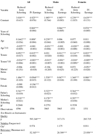
The results from the earnings function show that the return to schooling obtained using the IV method exceeds the return obtained using OLS. Thus, the returns to schooling obtained using IV (OLS) are 6.93 (4.72) per cent for the combined sample, 6.61 (4.36) per cent for the male sample, and 7.38 (5.26) per cent for the female sample. The Hausman test rejects the null hypothesis of equality of the OLS and IV estimates in each instance. The average difference between the IV and OLS estimates is 2.19 percentage points. Alternatively stated, the OLS estimates are 31.42 per cent less than the IV estimates. The IV estimates will be larger than the OLS estimates where measurement error is important, and where the instruments (education levels of the worker’s mother and father) are correlated with ability (Card, 1999). Card (1999, p.1842) argues that this type of finding is typical in the literature for advanced economies. Nevertheless, these family background instruments are popular in the literature, and the results obtained here are consistent with what is known from the rather large set of studies for other countries that adopt this approach.
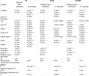
The second set of individual-type instruments uses information on preschool attendance and delayed primary school education. The reduced form regressions for schooling and the IV earnings function using these instruments are reported in Table 7.
The explanatory power for the first-stage estimations is fairly high, with the value of the R2 being between 0.1859 (combined sample) and 0.2070 (females). These values are,
however, well below the values reported in Table 6, where the parents’ levels of education were used as instruments, though they are more than double the level of explanation achieved using the natural instruments in Tables 4 and 5. This is consistent with Pons and Gonzalo (2002), who note that within the set of family background information they considered, parents’ education levels performed the best as instruments.
197
Table 6: Instrumenting Schooling with Parental Education
All Males Females
Variable
Reduced form
Schooling IV-Earnings
Reduced form Schooling IV-Earnings Reduced form Schooling IV-Earnings Constant 3.018*** (0.613) 4.925*** (0.076) 1.985*** (0.766) 4.985*** (0.093) 4.239*** (1.015) 4.619*** (0.131) Years of Schooling 0.069*** (0.004) 0.066*** (0.005) 0.074*** (0.005)
Age 0.1662*** (0.036) 0.008* (0.004) 0.239*** (0.044) 0.006 (0.005) 0.077 (0.060) 0.011 (0.008)
Age2/10 -0.025*** (0.005) -0.001 (0.001) -0.031*** (0.006) -0.001 (0.001) -0.020** (0.008) -0.001 (0.001)
Tenure 0.052*** (0.017) 0.015*** (0.002) 0.021 (0.020) 0.011*** (0.002) 0.114*** (0.030) 0.022*** (0.004)
Tenure2/10 -0.014*** (0.006) -0.003*** (0.001) -0.013* (0.007) -0.001* (0.001) -0.018* (0.009)* -0.005*** (0.001) Marital Status -0.006 (0.151) -0.002 (0.018) -0.196 (0.205) 0.040 (0.025) 0.072 (0.225) -0.051* (0.028)
Urban 1.486*** (0.103) 0.0568*** (0.015) 1.539*** (0.122) 0.047*** (0.018) 1.368*** (0.189) 0.088*** (0.026)
Female -0.099 (0.098) -0.196*** (0.012)
Father's Schooling 0.341*** (0.019) 0.323*** (0.023) 0.364*** (0.032) Mother's Schooling 0.218*** (0.021) 0.178*** (0.026) 0.297*** (0.038)
R2 0.2948 0.2751 0.3538
Observations 4596 4596 3065 3065 1531 1531
Test Results on Instruments
Quality
F 593.348*** 317.171 283.715
Validity (Sargan test)
Chi2 0.574 1.175 0.011
Relevance (Hausman test)
F 52.345*** 28.399*** 23.958***
198
TABLE 7: INSTRUMENTING SCHOOLING WITH PRESCHOOL ATTENDANCE AND DELAYED PRIMARY SCHOOL ENROLMENT
All Males Females
Variable
Reduced form
Schooling IV-Earnings
Reduced form
Schooling IV-Earnings
Reduced form
Schooling IV-Earnings
Constant 9.226*** (0.766) 4.962*** (0.078) 7.419*** (0.926) 5.009*** (0.095) 12.269*** (1.343) 4.677*** (0.137) Years of Schooling 0.062*** (0.006) 0.060*** (0.007) 0.066*** (0.008)
Age 0.273***
(0.038)
0.010** (0.004)
0.330*** (0.047)
0.008 (0.006) 0.210*** (0.067)
0.012 (0.008)
Age2/10 -0.037***
(0.005)
-0.001* (0.0001)
-0.041* (0.006)
-0.001 (0.001) -0.035*** (0.009)
-0.001 (0.001)
Tenure 0.037**
(0.018) 0.015*** (0.002) 0.004 (0.021) 0.011*** (0.002) 0.109*** (0.034) 0.023*** (0.004) Tenure2
/10 -0.013** (0.006) -0.003*** (0.001) -0.011 (0.007) -0.001* (0.001) -0.019* (0.011) -0.005*** (0.001) Marital Status -0.117
(0.162)
-0.003 (0.018)
-0.361* (0.217)
0.038 (0.025) 0.028 (0.249) -0.050* (0.028)
Urban 1.962***
(0.109) 0.073*** (0.018) 2.005*** (0.126) 0.060*** (0.022) 1.801*** (0.209) 0.106*** (0.029)
Female -0.158
(0.108) -0.196*** (0.012) Preschool Attendance 1.924*** (0.119) 1.8137*** (0.146) 2.068*** (0.203) Delayed Primary School Enrolment -0.743*** (0.067) -0.633*** (0.077) -1.009*** (0.127) R2
0.19 0.19 0.21
Observations 4596 4596 3065 3065 1531 1531
Test Results on Instruments
Quality
F 207.286*** 118.962*** 90.331***
Validity (Sargan test)
Chi2 1.047 0.699 0.566
Relevance (Hausman test)
F 8.611** 5.909** 2.863*
Notes: Standard errors in parentheses. *, ** and *** denote statistical significance at the 10 per cent, 5 per cent and 1 per cent levels, respectively.
Naturally, these instruments could be subject to the same limitation as the
parents’ levels of schooling, in that they could be correlated with the omitted ability
variable. However, it is noted that the literature on the links between school starting age and academic outcomes in advanced countries has reported mixed findings (Li and Miller, 2009), and so these instruments could be suitable from this perspective.
199
downwards by 23.9 per cent. The fact that the IV estimates exceed the OLS estimates can again be linked to what Card (1999) refers to as ability bias in this type of IV estimate. Hence, greater differences between the IV and OLS estimates are observed when individual-type instruments are used than when the cohort-type instruments are employed. The various sets of instruments are evaluated more formally in the following section.
INSTRUMENT QUALITY, VALIDITY, AND RELEVANCE
200
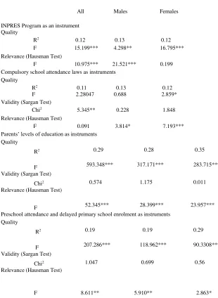
TABLE 8: QUALITY, VALIDITY, AND RELEVANCE OF THE INSTRUMENTS
All Males Females
INPRES Program as an instrument Quality
R2 0.12 0.13 0.12 F 15.199*** 4.298** 16.795*** Relevance (Hausman Test)
F 10.975*** 21.521*** 0.199 Compulsory school attendance laws as instruments
Quality
R2 0.11 0.13 0.12 F 2.28047 0.688 2.859* Validity (Sargan Test)
Chi2 5.345** 0.228 1.848 Relevance (Hausman Test)
F 0.091 3.814* 7.193*** Parents’ levels of education as instruments
Quality
R2 0.29 0.28 0.35
F 593.348*** 317.171*** 283.715*** Validity (Sargan Test)
Chi2 0.574 1.175 0.011 Relevance (Hausman Test)
F 52.345*** 28.399*** 23.957*** Preschool attendance and delayed primary school enrolment as instruments
Quality
R2 0.19 0.19 0.29
F 207.286*** 118.962*** 90.3308*** Validity (Sargan Test)
Chi2 1.047 0.699 0.56 Relevance (Hausman Test)
F 8.611**
5.910** 2.863*
201
The final criterion is relevance. The relevance of the instrument is examined using the Hausman test of whether the OLS and IV estimates differ significantly (Hausman, 1978). This study finds that when using parents’ education as instruments, or when using preschool attendance and delayed primary school enrolment as instruments, the results for all samples show that the endogeneity of schooling significantly affects the estimated return to schooling. When instrumenting schooling using the compulsory school attendance laws, the Hausman test appears to confirm the necessity to use an IV approach in the male and female samples. Recall, however, that the IV estimates of the return to schooling in these samples were imprecisely determined, and in the case of females, incorrectly signed, and it is these perverse outcomes results that are behind the outcome for the Hausman test. Pons and Gonzalo (2002) have a similar result in their study of male workers in Spain, and they attribute this to “the correlation between these instruments and the years of schooling is not strong enough to accurately estimate the returns to schooling” (Pons and Gonzalo, 2002, p.757). For similar reasons, the INPRES program is unsatisfactory as an instrument in this more recent data collection.
The difference between the OLS and IV estimates is more apparent in these analyses in the estimations based on instruments that vary across individuals in a given age category than it is for the instruments that are the same for all individuals in a given age category. This result is in line with research by Levin and Plug (1999), Li and Luo (2004), Lemke and Rischall (2003), and Poms and Gonzalo (2002). Where there is a significant difference between the IV and OLS estimates, the difference is greater than that which is usually associated with measurement error. Card (1999) suggests a 10 percent bias from errors in variables, though the reliability of the schooling variable could be less (and so the measurement error bias greater) in Indonesia than in developed countries. Only the conventional instruments of parental education, pre-school attendance, and delayed primary school enrolment, pass the standard criteria of quality, relevance and validity. It would seem that this pattern is attributable to the variables that vary across individuals being correlated with the omitted ability variable, rather than with ability being important in wage determination. Any strengthening of this correlation over the past two decades will be linked to sorting with the schools system rather than with labour market outcomes.
CONCLUSIONS AND POLICY IMPLICATIONS
This article presents evidence on the returns to schooling in Indonesia and highlights
several policy implications. First, the estimated returns to education in Indonesia are
202
considered based on the costs of education (both the direct costs and the true opportunity costs of education) following Barouni and Broecke, (2014).
Second, we also find evidence of high earning inequalities between male and female and also between rural and urban regions. Policy initiatives by both the central government and local government of Indonesia should be focussed on equal opportunity both in the private and public sectors.
Finally, it is extremely important to measure the rate of returns to education for better understanding of education and training investments. However, this should not be based on the quantitative measures alone; rather much more priority should be given to qualitative information concerning the quality of schooling, teachers, and so on, and relevance of the education or training that is being delivered. Bennell (1998) also emphasized on this. Thus, a clear understanding of the factors affecting returns to education can serve as an effective tool in the hands of organizations and institutions dealing with transition from school to work.
ACKNOWLEDGEMENT
We acknowledge financial assistance from the Department of Foreign Affairs and Trade (DFAT), through the Australian Development Research Awards Scheme (ADRAS). However, the views and interpretations expressed in this article are those of the authors. They do not in any way implicate the views and policies of the Australian Government. We are also grateful to late Professor Paul Miller, School of Economics & Finance, Curtin University for his detail comments and suggestions on the earlier version of this paper.
ENDNOTES
1. Card (1999) reviews various limitations of the IV approach. Consideration of alternative sets of instruments has appeal in view of these limitations, and this is the strategy we adopt in the empirical section of this paper.
2. In 1973, the Indonesian government launched a major school construction program, the Sekolah Dasar (Primary Schools) INPRES program. INPRES stands for Instruksi Presiden (Presidential Instruction). Between 1973-74 and 1978-79, more than 61,000 primary schools were constructed, an average of two schools per 1,000 children aged 5 to 14 in 1971.
REFERENCES
Aromolaran, A.B. (2006) Estimates of Mincerian Returns to Schooling in Nigeria. Oxford Development Studies, 34(2): 265-292.
Ashenfelter, O., and A. Krueger. (1994) Estimates of the Economic Return to Schooling from a New Sample of Twins. American Economic Review, 84(5): 1157-1173.
Aslam, M., F. Bari, and G. Kingdon. (2012) Returns to Schooling, Ability and Cognitive Skills in Pakistan. Education Economics,20(2): 139-173.
203
Behrman, J.R., and A.B. Deolalikar. (1993) Unobserved Household and Community Heterogeneity and the Labor Market Impact of Schooling: A Case Study for Indonesia. Economic Development and Cultural Change, 41(3): 461-488.
Bennell, P. (1998). Rates of Return to Education in Asia: A Review of the Evidence. Education Economics, 6(2):107-120.
Cheidvasser, S., and H.B. Silva. (2007) The Educated Russian’s Curse: Returns to Education in the Russian Federation during the 1990s. Labour, 21(1): 1-41.
Card, D. (1999) The Causal Effect of Education on Earnings. Chapter 30 in Handbook of Labor Economics, Vol. 3, edited by O. Ashenfelter and D. Card, Elsevier Science.
Chapman, B. (1997) Conceptual Issues and the Australian Experience with Income Contingent Charges for Higher Education. Economic Journal, 107(442): 738-51.
Comola, M., and L. de Mello. (2010) Educational Attainment and Selection into the Labour Market: The Determinants of Employment and Earnings in Indonesia. Paris School of Economics Working Paper, No. 2010-06, Paris.
Deolalikar, A.B. (1993) Gender Differences in the Returns to Schooling and in School Enrollment Rates in Indonesia. The Journal of Human Resources, 28(4): 899-932. Duflo, E. (2001) Schooling and Labor Market Consequences of School Construction in Indonesia: Evidence from an Unusual Policy Experiment. The American Economic Review, 91(4): 795-813.
Flabbi, L., S. Paternostro, and E.R. Tiongson. (2008) Returns to Education in the Economic Transition: A Systematic Assessment using Comparable Data. Economics of Education Review, 27(6): 724-740.
Flanagan, R. J. (1998) Were Communists Good Human Capitalist? The Case of the Czech Republic. Labour Economics, 5: 295-312.
Hausman, J.A. (1978). Specification Tests in Econometrics. Econometrica, 46: 1251-1271.
Jamison, D.T., and J.V.D. Gaag. (1987) Education and Earnings in the People’s Republic of China. Economics of Education Review, 6 (2), pp. 161-166.
Kalinowski, T. (2007) Democracy, Economic Crisis, and Market Oriented Reforms: Observation from Indonesia and South Korea since the Asian Financial Crisis. Comparative Sociology, 6: 344-373.
Kazianga, H. (2004) Schooling Returns for Wage Earners in Burkina Faso: Evidence from the 1994 and 1998 National Surveys. Economic Growth Center Discussion Paper, No. 892, Yale University, New Haven, CT.
Lemke, R.J., and I.C. Rischall. (2003) Skill, Parental Income, and IV Estimation of the Returns to Schooling. Applied Economics Letters, 10 (5): 281-286.
204
Li, H., and Y. Luo. (2004) Reporting Errors, Ability Heterogeneity, and Returns to Schooling in China. Pacific Economic Review, 9 (3): 191-207.
Li, I. and P.W. Miller. (2009) Academic Performance and Graduate Outcomes: Does Age Matter? In E. Balistrieri and G. DeNino (eds) New Research in Education: Adult, Medical and Vocation, Nova Science Publishers, Inc, New York, pp. 1-25.
Pons, E. and Gonzolo, M.T., (2002). Returns to Schooling in Spain: How Reliable are Instrumental Variable Estimates? Labour, 16 (3): 747-770.
Psacharopoulos, G. (1981) Returns to Education: An Updated International Comparison. Comparative Education, 17 (3): 321-341.
Psacharopoulos, G. (1994) Returns to Investment in Education: A Global Update. World Development, 22 (9): 1325-1343.
Puhani, P.A. (2000) The Heckman Correction for Sample Selection and its Critique. Journal of Economic Surveys, 14 (1): 53-68.
Purnastuti, L., P.W. Miller and R. Salim. (2013) The Evolution of Labour Market Returns to Education in Indonesia: Evidence from the Family Life Survey. Bulletin of Indonesian Economic Studies, 49 (2): 213-236.
Qian, X., and R. Smyth. (2008) Private Returns to Investment in Education: An Empirical Study of Urban China. Post-Communist Economies, 20(4): 483-501.
Ren, W., and P.W. Miller. (2012) Changes Over Time in the Return to Education in Urban China: Conventional and ORU Estimates. China Economic Review, 23(1): 154-169.
Stolzenberg, R.M., and D.A. Relles. (1997) Tools for Intuition about Sample Selection Bias and its Correction. American Sociological Review, 62: 494-507.