Using variation in schooling availability to estimate
educational returns for Honduras
Arjun S. Bedi
a, Noel Gaston
b,*aInstitute on East Central Europe, Columbia University and CEEERC, Warsaw University, Warsaw, Poland
bSchool of Business, Bond University, Gold Coast, Queensland 4229, Australia
Received 1 February 1997; accepted 8 January 1998
Abstract
This paper presents IV estimates of the returns to schooling for Honduran males by exploiting the variation in the availability of schooling at the time individuals were eligible to commence their education. The IV estimates are significantly higher than OLS estimates. The higher rate of return estimates are driven by the greater schooling attain-ment and the higher marginal returns for individuals from more privileged family backgrounds. In line with studies for developed countries, we conclude that, when estimating rates of return to education for developing countries, it is important to account for the endogeneity of educational attainment. [JEL J31, J24, O15]1998 Elsevier Science Ltd. All rights reserved.
Keywords: Returns to education; School availability; Educational attainment
1. Introduction
Innumerable studies using data from all parts of the world estimate that educational rates of return for an additional year of schooling are positive and range any-where from 5 percent in developed countries to as high as 29 percent in developing countries.1Armed with esti-mates such as these, developing countries like Honduras have allocated substantial portions of their budgets to the education sectors.2While rate of return estimates are an important ingredient in policy-making, as is well known, they suffer from several drawbacks. For example, rate of return estimates are biased when individual heterogen-eity and the endogenheterogen-eity of schooling investment
* Corresponding author. E-mail: noel [email protected] 1A survey of returns to education in developing countries, focusing on Latin America in particular, is provided by Psachar-opoulos and Ng (1992).
2In 1995, public spending on education accounted for approximately 16 percent of total government expenditure in 64 developing countries (UNDP, 1995).
0272-7757/98/$ - see front matter1998 Elsevier Science Ltd. All rights reserved. PII: S 0 2 7 2 - 7 7 5 7 ( 9 8 ) 0 0 0 1 3 - 2
decisions is not taken into account. The point is that edu-cational outcomes are not assigned randomly across the population, instead years of education may be determ-ined through a process of self-selection. Thus, relying on ordinary least squares (OLS) may result in incorrect estimates of the actual return to education.
and Zimmerman (1993) report slightly lower educational return estimates compared with conventional OLS esti-mates.
A second broad approach relies on constructing a “sel-ectivity-correction” term from a schooling attainment equation and including the correction term in the earn-ings equation to obtain consistent estimates of edu-cational returns. Studies using this strategy typically report higher returns compared with OLS estimates (e.g., Gaston and Tenjo, 1992; Bedi and Gaston, 1997). A third, recent, and perhaps more convincing approach, relies on using exogenous (or “natural”) variation in edu-cational attainment to provide instrumental variables (IV) estimates of the returns to education. This approach relies on finding a variable or set of variables that influ-ence schooling decisions but do not affect earnings out-comes. Card (1993) provides a review of studies that have applied this methodology. Most of these IV studies also yield significantly higher estimates of the returns to schooling (e.g., Harmon and Walker, 1995), although there are some that have not (e.g., Angrist and Krueger, 1991).
Most of the studies cited above have relied on data from developed countries. Despite the policy impli-cations, there is limited evidence on how returns to edu-cation are affected by the endogeneity of eduedu-cation in developing countries. Unfortunately, panel data on twins or satisfactory measures of ability are not common for developing countries. This paper is in the spirit of the third approach and presents IV estimates of educational returns for a developing country. In particular, we use recently collected survey data from Honduras and rely on variation in the educational distribution of individuals caused by fluctuations in the availability of schooling to provide identifying information for individuals’ school-ing decisions.
In Section 2, we discuss the empirical approach that is used to estimate the returns to education. In Section 3, we describe the data and our estimates. A discussion of the results and concluding comments are presented in Section 4.
2. The empirical approach
Consider the following model that consists of an earn-ings equation and a schooling equation
Yi5b9xXi1bsSi1ei (1)
Si5d9zZi1ni, (2)
where for each individual i, Yiis the natural logarithm
of earned income and Xi is a vector of human capital
and demographic variables. Sirepresents years of
school-ing and Ziis a vector of schooling attainment
determi-nants. The error termseiandniare normally distributed
with zero means and positive variances.
As is well known, OLS estimates of bs and bx are
consistent only ifeiandniare uncorrelated. However, if
an unobserved characteristic, say “ability”, has a positive effect on earnings and schooling then OLS estimates of the return to schooling will be biased upward. On the other hand, measurement error in schooling may gener-ate a negative correlation between the two error terms and induce a negative bias in OLS estimates (see Gril-iches, 1977; Blackburn and Neumark, 1995). Further, as pointed out by Griliches (1977), unobserved factors that have a positive impact on labour market success may lead to lower schooling attainment (and cause OLS esti-mates to be biased downward). This latter case suggests that individuals with greater earnings potential at each level of education invest less in schooling, since they have a higher opportunity cost of schooling. A negative bias could also arise if, contrary to a comparative advan-tage story, those with low schooling have a higher earn-ings capacity (and higher returns to schooling) but cur-tailed their education due to higher discount rates. Such a negative correlation is implied by the Becker model of human capital investment in which schooling is acquired until the marginal return to schooling equates the dis-count rate (see Card, 1995). Thus, while unobserved ability may bias the OLS estimates upwards, allowing for the endogeneity of schooling may impart a downward bias on the conventional OLS rate of return estimates. The overall size and sign of the bias are, of course, theor-etically indeterminate and need to be resolved empiri-cally.
To obtain consistent coefficient estimates for Eq. (1), we rely on IV estimation. (Appendix A provides esti-mation details.) We use the variation in schooling avail-ability (SA) as an instrument.3 More specifically, our measure of SA is the number of primary school teachers per capita.4The number of teachers is likely to be highly
3For each individual in the sample, we construct a time-line to determine the year in which the individual entered school (assuming that school starts at 7 years of age, the legal school starting age in Honduras). Individuals are then matched to the SA measure for that year. SA has a mean of 4.01 and ranges between 2.38 and 4.52.
Fig. 1. School availability in Honduras.
correlated with the contraction and expansion of the schooling sector in Honduras. While there has been an overall improvement in the availability of schooling in Honduras since World War II, Fig. 1 reveals that the growth in SA has not been uniform over time. There were relatively steep increases in SA up to the early 1960s, but these were followed by relative decline and stagnation in the mid-1960s and 1970s. However, with the advent of democracy, a period of relative political stability, and the primary education expansion projects financed by USAID (for further details, see Bedi, 1996), the 1980s witnessed a sustained increase in SA. By 1982, SA had recovered to its 1965 level and soon after reached its highest level (in 1985, SA was around 5.18).5 The use of variation in SA over time as an instrument for years of schooling is similar to the use of changes in compulsory schooling laws over time by Harmon and Walker (1995). Students who grew up during periods of higher educational availability and access to schooling are likely to have faced lower educational costs and consequently, should have acquired more education. This is borne out by the data. The correlation between actual schooling and SA is 0.16 and individuals educated dur-ing a time with above average SA have 1.44 more years of schooling than those educated at a time of low SA.
3. The data and results
The data for our study are from the May 1990 survey of Honduran households conducted by the Office of
5The youngest person in our sample was born in 1974, so that only the SA data up to 1981 are used (see footnote3).
Planning Co-ordination and Budget. This survey consti-tutes the primary data collection effort by the Honduran government and is designed to provide a random sample with a national scope. It includes general information on the condition of the household as well as specific infor-mation on the education, occupation, and earnings characteristics of each household member.
We restrict our sample to males aged between 16 and 64, who are not currently full-time students, who supply information on their labour income and for whom we have information on family background. In addition, domestic servants were excluded because their recorded earnings are probably underestimated due to payments-in-kind. The sample consists of 2014 individuals.6The descriptive statistics for the variables are listed in Table 1. Individuals in the sample average less than five years of schooling and have average labour market earnings of 256 lempiras (or $US 64 in 1990).
3.1. Estimates of the earnings and schooling equations
Column 1 of Table 2 displays OLS estimates of Eq. (1). The coefficients indicate positive educational returns of 6.1 percent and positive, concave returns to age. (We use age rather than experience, because experience may
Table 1
Descriptive statistics
Variable Label Mean Std. Dev.
LOGEARN (Y) Log of monthly earnings in lempiras 5.22 0.81
SCHOOL (S) Years of schooling 4.74 3.55
AGE Age 24.50 7.98
URBAN Dummy, San Pedro Sula or Tegucigalpa51 0.34 0.47
SOUTH Dummy, Resides in the South51 0.08 0.27
SWEST Dummy, Resides in the Southwest51 0.08 0.27
NORTH Dummy, Resides in the North51 0.06 0.25
NWEST Dummy, Resides in the Northwest51 0.32 0.46
NEAST Dummy, Resides in the Northeast51 0.06 0.24
WEST Dummy, Resides in the West51 0.09 0.28
CENTRAL Dummy, Resides in the Central region51 0.29 0.45
SCHHEAD Years of schooling of household head 2.47 3.25
SCHSPSE Years of schooling of spouse of household head 1.27 3.25
SCHOOL AVAILABILITY Primary school teachers per 1000 population 4.01 0.44 (SA)
Notes: Observations52014. The population data were obtained from various issues of Economic Survey of Latin America and the
Caribbean, United Nations, Santiago, Chile, and Economic and Social Progress in Latin America, Inter-American Development Bank,
Washington D.C. Data for SA are from several issues of the UNESCO Year Book of Education.
Table 2
Earnings and schooling equations
Variable (1) (2) (3)
Earnings Schooling Earnings
OLS Reduced form IV
Intercept 4.021 (0.144) 21.851 (1.041) 3.931 (0.160)
S 0.061 (0.005) – 0.169 (0.073)
SA – 0.754 (0.234) –
AGE 0.041 (0.009) 0.147 (0.043) 0.020 (0.017)
AGE2*100 20.051 (0.014) 20.230 (0.074) 20.013 (0.029)
URBAN 0.400 (0.037) 1.476 (0.161) 0.236 (0.117)
SOUTH 20.297 (0.063) 20.766 (0.273) 20.215 (0.085)
SWEST 20.219 (0.063) 20.191 (0.693) 20.195 (0.067)
NWEST 20.029 (0.039) 20.141 (0.824) 20.013 (0.032)
NORTH 0.132 (0.068) 0.095 (0.321) 0.121 (0.070)
NEAST 0.119 (0.069) 20.090 (0.298) 0.126 (0.071)
WEST 0.051 (0.061) 21.287 (0.264) 0.193 (0.114)
SCHHEAD 0.025 (0.005) 0.328 (0.023) 20.011 (0.025)
SCHSPSE 0.020 (0.006) 0.167 (0.028) 0.002 (0.014)
F 74.84 73.61 59.62
R2 0.309 0.306 0.263
Notes: sample size52014. Standard errors in parentheses. have introduced an additional source of endogeneity.) Compared with the 17.2 percent return reported in Psa-charopoulos and Ng (1992) our estimates seem very low. However, the apparently low OLS returns are readily explained by differences in the specifications and sample used. Psacharopoulos and Ng use 1989 data, limit their attention to an urban sample, use an extremely
parsi-monious specification and use the sum of wage income and self-employment income as the earnings variable. In fact, using a model specification and sample restrictions as similar as possible to Psacharopoulos and Ng, we find educational returns of around 14 percent.
with estimates from studies on other Latin American countries (e.g., Heckman and Hotz, 1986). To the extent that parental education is correlated with inherited ability, we find that inclusion of parental education low-ers educational returns from 7.3 percent (reported in Table 3) to 6.1 percent. This suggests that in the absence of controls for ability, OLS estimates will suffer from an upward bias.
Estimates of Eq. (2) appear in column 2 of Table 2. As expected, living in a major city, the schooling of the household head and the spouse of the household head are positively related to educational attainment. Of primary interest is the sign and the magnitude of the coefficient on SA. The coefficient is statistically significant and has the anticipated positive sign. The size of the coefficient is also noteworthy — growing up during periods of greater schooling availability is associated with higher edu-cational attainment. An increase in schooling availability from say, three teachers to four teachers per capita increases educational attainment by about three-quarters of a year.
The IV estimates of the earnings function appear in column 3 of Table 2. The estimate of the return to edu-cation is 16.9 percent. This is more than two and a half times the corresponding OLS estimate. This implies that there is a negative correlation between the errors in the earnings equation and the schooling equation. Interest-ingly, the size and sign of the bias in OLS estimates are consistent with the recent developed country literature. For example, using data from the United Kingdom and a similar methodology to that employed here, Harmon and Walker (1995) report estimates that are 9 percentage
Table 3
Impact of alternative specifications on educational returns
OLS IV
1. Baseline specification 0.061 (0.005) 0.169 (0.073)
Alternative schooling models
2. Selectivity model — continuous schoolinga 0.061 (0.005) 0.169 (0.071)
3. Tobit model for schoolinga 0.061 (0.005) 0.124 (0.026)
4. Ordered probit model for schoolinga,b 0.061 (0.005) 0.106 (0.012)
Alternative earnings models
5. Exclude schooling of household head and spouse 0.073 (0.004) 0.147 (0.012)
6. Include industrial sector dummiesc 0.056 (0.005) 0.157 (0.072)
7. Include occupational dummiesd 0.052 (0.005) 0.158 (0.072)
8. Urban sample onlye 0.064 (0.005) 0.188 (0.114)
Notes: N5 2014. Standard errors in parentheses. The reported estimates are the coefficients on schooling in the OLS and the IV model. Earnings and schooling equations included variables that appear in Table 2, except where indicated.
aSee Appendix A for details.
bThe dependent variable consists of five categories for years of schooling: 0 years, 2 or 3 years, 4 or 5 years, 6 years, and more than 6 years.
cThe sectors are manufacturing, service, construction, utilities, and agriculture. dThe occupational groups are professional, agricultural, skilled, unskilled, and other. eSample size5948.
points higher than OLS estimates (their estimates jump from 6.1 percent to 15.2 percent). Increases in magnitude of between 50 to 60 percent are also reported in papers relying on data from the United States (see Card, 1995).
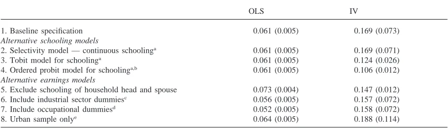
3.2. Alternative model specifications
Table 3 presents a summary of the schooling rate of return estimates for alternative model specifications that were estimated to investigate the sensitivity of our results. Row 1 presents OLS and IV estimates from the baseline specification reported in Table 2. These rate of return estimates are best interpreted as estimates for a randomly-selected individual. Rows 2, 3, and 4 display selectivity-bias corrected estimates based on different assumptions about observed years of schooling. That is, these rate of return estimates are for individuals given their observed schooling choices. Appendix A provides details of the estimation procedures.
Table 4
Further specification tests
Schooling SA
1. OLS estimate 0.061 (0.005) –
2. IV estimate 0.169 (0.073) –
3. Reduced form earnings – 0.128 (0.055)
4. SA in the earnings equation 0.060 (0.005) 0.082 (0.054)
5. Using SA — household head has no education interaction in 0.152 (0.093) 0.013 (0.089) schooling equation
6. Using SA — family education interactions in schooling equationa 0.198 (0.234) 20.022 (0.185)
Notes: N52014. Standard errors in parentheses. The reported estimates are the coefficients on SA and SCHOOL in the earnings equation. Models included age, age-squared, dummies for living in a city, region of country, schooling of household head and spouse of household head.
aInteractions of SA and schooling of household head (SCHHEAD) and schooling of spouse of household head (SCHSPSE).
Again, although lower than the baseline estimate it is still significantly higher than the OLS estimate.
Rows 5, 6, and 7 present alternative specifications of Eq. (1) that respectively, exclude information on school-ing of household head and spouse of household head, include industrial sector dummies, and include occu-pational categories.7 The results for these models also confirm the conclusions reached above. Finally, out of concern for the stark rural/urban differences in a country such as Honduras, we estimate Eqs. (1) and (2) on a geographically more homogeneous sample, i.e., those living in the two major cities of Tegucigalpa and San Pedro Sula. The gap between the OLS and IV estimates for this sample is similar to earlier estimates.8Overall, the ratios of the IV and OLS point estimates for rows 5 through 8, lie between 2.0 and 3.0.
3.3. Is school availability a valid instrument?
For our measure of school availability to be a valid instrument for years of schooling, SA must influence educational decisions but be uncorrelated with the unob-served factors influencing earnings. However, if the increase in school availability is viewed as an increase in school quality, exclusion of SA from the earnings equ-ation may be inappropriate (see Card and Krueger, 1996). Individuals who were educated during a time per-iod in which school quality was higher may have higher earnings than those educated in a time of lower school quality.
Table 4 presents results of some additional
specifi-7Some authors have argued that occupation is endogenous and should be excluded from earnings regressions (e.g., Knight and Sabot, 1981).
8Although imprecise, estimates using the non-urban sample yield similar increases in education returns: OLS, 0.049 (standard error 0.009) and IV, 0.154 (standard error 0.151).
cations designed to examine the effect of excluding SA from the earnings equation. Rows 1 and 2 display the OLS and IV rate of return estimates reported in Table 2. Row 3 displays the estimates from the reduced form earnings equation and row 4 a model specification with SA added to Eq. (1). In the latter case, the estimated coefficient on schooling is virtually identical to the base-line OLS estimate and there is a statistically insignificant coefficient sign on SA, suggesting that it is not an omit-ted variable in the earnings equation.
The increasing availability of schooling is expected to lower the cost of schooling for all households. However, the lower costs of schooling may have a greater impact on children from low income households or those that lack sufficient funds necessary to finance their education. This suggests an alternative set of instruments for schooling. In an attempt to capture low income house-holds we followed Card (1993) and included SA in the earnings function and created an additional variable by interacting SA with a dummy for head of household hav-ing no education. Results from this specification are dis-played in row 5. The educational return estimates are similar to our baseline estimate, but not very precise. The point estimate of the effect of SA on earnings is statistically insignificant.
Finally, we conduct additional tests suggested by Bound et al. (1995) to check the performance of our instrument. The quality of the instrument can be gauged by two indicators: (i) an F-test on excluding the instru-ments from the reduced form schooling equation should be rejected and (ii) the inclusion of the instrument should increase the adjusted R2of the reduced form schooling equation. The F-test for excluding our instrument recorded a p-value of 0.0013, indicating its high statisti-cal significance. Further, the addition of SA to the schooling equation raised the adjusted R2 by 0.0033.9 These results indicate that the SA instrument performs well. Together, the results summarised in Table 4 and these tests suggest that the inclusion of SA as an exogen-ous determinant of schooling attainment and the exclusion of SA from the earnings equation are not unreasonable.
4. Discussion and conclusion
The results in this paper suggest that ignoring the endogeneity of education leads to a substantial under-statement of the returns to education. We examined the endogeneity issue in the education–earnings relationship by instrumenting years of schooling with a measure of schooling availability at the time individuals commenced their schooling (SA). Using recently collected household survey data for Honduran males, we found that account-ing for the endogeneity of schoolaccount-ing decisions leads to educational returns that are two to three times higher than OLS estimates of returns to education.
The estimates of returns to education were robust to several changes in specification. Further, we used inter-actions between SA and family education as instruments in earnings models that included the SA variable. The results of these specifications did not provide any evi-dence that would lead us to reject the use of SA as an exogenous determinant of schooling.
Although the results presented in this paper are similar to work that relies on including a “selectivity-correction” term in the earnings equation, we found the current approach more convincing. For example, Bedi and Gas-ton (1997) relied on excluding family background vari-ables from the earnings equation to achieve identifi-cation. Imposing exclusion restrictions of this sort seems inappropriate. The use of exogenous variation in school-ing availability freed us from imposschool-ing potentially inap-propriate restrictions and allowed us to delve deeper into the underlying reasons for the higher rate of return esti-mates.
A possible explanation for the higher rate of return
9The partial regression of school on SA (controlling for all other variables) yielded a partial adjusted R2of 0.0046.
estimates is that OLS estimates are downward-biased due to measurement error in the schooling variable. However, it is unlikely that the large gap between the OLS and IV estimates can be explained solely by measurement error. A theoretical explanation for the higher IV estimates is “discount rate bias” (see Card, 1993). The IV estimate of educational returns is simply the ratio of the differences in average wages and average education (controlling for other variables) between indi-viduals affected by a particular schooling intervention and those unaffected by the intervention.10A schooling intervention may take the form of changes in the mini-mum school leaving age, the location of a school in a certain geographic area, or changes in the availability of schooling. The IV estimates depend on the marginal return to schooling for the group that is most affected by the increase in the availability of schooling. If changes in schooling availability affect a group with a sufficiently high marginal return to schooling, then the IV estimate will exceed the conventional OLS estimate. If the increase in the availability of schooling induces individ-uals with a low propensity for education to increase their schooling, the estimated return to education will reflect the marginal returns for the low-education group. This marginal return might be higher than the average return to schooling for the population as a whole if people with low education have high discount rates and limited access to funds to finance education, rather than low ability. This explanation is contrary to the more conven-tional view that individuals with less schooling have lower ability and low returns to schooling. On the other hand, if changes in school availability induce individuals in the high-education group to acquire even more edu-cation, then the associated return will reflect the marginal return to schooling for the high education group. If schooling decisions are largely influenced by compara-tive advantages and differences in ability then individ-uals acquiring more education will have higher returns to education than those with fewer years of education. Thus, IV estimates based on the marginal returns to schooling for the high education group could also exceed the average return to schooling for the population as a whole.
Clues on the mechanism underlying the increase are provided by the pattern of signs on the interaction of SA with the education of the head of the household in the schooling attainment equation. The sign on the interac-tion term is negative and significant, implying that the coefficient on SA is smaller for individuals from “poor”
family backgrounds.11
As argued by Willis and Rosen (1979) family background may be considered a reason-able proxy for discount rates. This interpretation suggests that the increase in school availability has a smaller impact on educational attainment for individuals with higher discount rates (i.e., those from poor family backgrounds) compared with those from “better” family backgrounds. Thus, it appears that the higher IV esti-mates are driven by higher marginal returns among the more educated. This in turn, at least for our sample, sug-gests that individual heterogeneity and comparative advantage were more important than differences in dis-count rates and schooling opportunities in shaping edu-cational outcomes.
A reason for the higher marginal returns among the more highly-educated may lie in the economic changes taking place in Honduras during this time period. The advent of democracy in 1980 was accompanied by rapid economic changes and a policy of trade liberalisation. These structural reforms may have increased the demand for skilled workers and caused an increase in the edu-cational return for the more highly educated. Recent work on diverse economic environments emphasises the link between increasing educational returns for the more highly-educated during periods of rapid economic and technical change. For example, Rutkowski (1996) found that, for Poland, the increase in educational returns after 1990 accrued largely to the more educated. Similarly, Foster and Rosenzweig (1996) have shown that the increase in human capital returns in areas affected by the Green Revolution in India, a period of rapid technical change, was also concentrated among the more educated. A better understanding of the process of educational determination and the impact of economic changes will certainly enhance our understanding of the factors under-lying the increase in IV estimates of the returns to edu-cation. However, regardless of the underlying mech-anism, our paper highlighted the importance of accounting for the endogenous nature of the schooling decision when attempting to obtain reliable estimates of educational rates of return. This is especially important for developing countries where the increasing scarcity of public funds and the tightening of foreign aid have increased the need for an accurate evaluation of edu-cational priorities.
11Specifically, we interact SA with a dummy for the house-hold head having zero years of education. This yielded an esti-mated coefficient on SA of 0.783 (standard error50.234) and an estimated coefficient on the interaction term of 2 0.117 (standard error50.046).
Acknowledgements
Bedi thanks the Mellon foundation for a grant that supported travel to Honduras. Both authors would like to thank Hessel Oosterbeek, Jenny Williams, and an anonymous referee for their constructive comments. The views expressed in this paper are solely attributable to the authors.
where all notation is as defined in the text and S*
i is a
latent variable underlying educational attainment. Observed and latent years of schooling are linked by a “censoring function” h, i.e., Si5h(S
*
i) (see Vella, 1993).
In addition, the p31 vector Ziis related to the q31
vector Xithrough the identity
Xi5J9Zi, (A3)
where J is a matrix consisting of zeros and ones, which selects a subset of Zi. The parameters of Eq. A(1) cannot
be estimated without some additional assumptions. These are
(a) (niuZi)|N(0,1).
(b) (eiuni,Zi)|N(0,1).
Hence, conditional on Zi,
S
eiAssumption (c) is the familiar rank condition for ident-ifying the parameters of a structural equation with an endogenous variable and is satisfied when Ziincludes at
least one variable excluded from Xi. Assumption (b)
places our model in the framework of simultaneous equ-ation models with a latent structure (e.g., Heckman, 1978; Vella, 1993).
We consider two alternative estimation methods. Method 1: Assume that schooling is observed and take expectations of Eq. A(1) conditional on Zi(and hence,
on Xi)
E(YiuZi)5b9xXi1bsE(SiuZi)1E(eiuZi). (A4)
First, note that a consistent estimate ofdzcan be obtained
from Eq. A(2), i.e., a consistent predictor is Sˆi5dˆz9Zi.
Secondly, since E(eiuZi)50, consistent estimates ofbs
using Method 1 are referred to as IV estimates in this paper. Of course, when S*
i is observed this is equivalent
to two-stage least squares estimation (e.g., Angrist and Krueger, 1991).
Method 2: Take expectations of Eq. A(1) and Eq. A(2) conditional on Ziand Si:
E(YiuZi,Si)5b9xXi1bsSi1E(eiuZi,Si) (A5)
E(S*
iuZi,Si)5d9zZi1E(niuZi,Si). (A6)
The procedure used to obtain consistent estimates ofbs
depends on the form of censoring: (i) S*
i is uncensored (e.g., Garen, 1984; Gaston and
Tenjo, 1992), then
E(niuZi,Si)5Si2dˆ9zZi5nˆi. (A7)
From (b), note that E(eiuZi,Si)5vE(niuZi,Si), so that
E(YiuZi,Si)5b9xXi1bsSi1vnˆi. (A8)
Hence, using the estimated OLS residual, nˆi, as an
additional regressor in Eq. A(1) will provide consistent estimates ofbs(andbx). Also, note thatv 5 sen/snn.
(ii) Tobit censoring (e.g., Bedi and Gaston, 1997), i.e.,
Si5
H
the maximum likelihood estimates ofdz andsnn). Iiis
an indicator function that equals 1 if Si is uncensored
and zero otherwise. Eq. A(9) is the conditional error term or “generalised residual” for each i (see Gourieroux et al., 1987). Similarly to (i), including the generalised residual as a regressor in Eq. A(1) provides a consistent estimate ofbs.
(iii) Years of education as a discrete ordered variable (e.g., Harmon and Walker, 1995; Vella and Gregory, 1996), i.e.,
where n50,1,2,.... Now create n dummy variables as follows
Dni5
H
1, if Dni5n
0, otherwise
Then the generalised residual is
E(niuZi,Dni)5DnipˆniPˆ−
1
ni(12 Pˆni)−
1
(Dni2 Pˆni), (A10)
where Pˆni is the estimated probability that individual i
is in category n, whilepˆniis the estimated value of the
density at that point (see Vella, 1993). When schooling is dichotomous (e.g., high school or more than high school as in Willis and Rosen, 1979), then Eq. A(10) simplifies to the familiar “inverse Mills ratio”.
References
Angrist, J.D., Krueger, A.B., 1991. Does compulsory school attendance affect schooling and earnings? Quarterly Journal of Economics 106, 979–1014.
Ashenfelter, O., Krueger, A.B., 1994. Estimates of the econ-omic return to schooling for a new sample of twins. Amer-ican Economic Review 84, 1157–1173.
Ashenfelter, O. and Zimmerman, D. (1993) Estimates of the return to schooling from sibling data: fathers, sons, and bro-thers. Working Paper No. 4491, National Bureau of Econ-omic Research, Cambridge.
Bedi, A. S. (1996) Essays on the influence of selection and school quality on earnings and educational attainment. Unpublished Ph.D. dissertation, Tulane University. Bedi, A.S., Gaston, N., 1997. Returns to endogenous education:
the case of Honduras. Applied Economics 29, 519–528. Blackburn, M., Neumark, D., 1995. Are OLS estimates of the
return to schooling biased downward? Another look. Review of Economics and Statistics 77, 217–229. Bound, J.D., Jaeger, A., Baker, R., 1995. Problems with
instru-mental variables estimation when the correlation between instruments and the endogenous explanatory variable is weak. Journal of the American Statistical Association 90, 443–450.
Card, D. (1993) Using geographic variation in college proxim-ity to estimate the return to schooling. Working paper no. 317, Industrial Relations Section, Princeton University. Card, D., 1995. Earnings, schooling and ability revisited.
Research in Labor Economics 14, 23–48.
Card, D., Krueger, A.B., 1996. School resources and student outcomes: an overview of the literature and new evidence from North and South Carolina. Journal of Economic Per-spectives 10, 31–50.
Foster, A.D., Rosenzweig, M.R., 1996. Technical change and human-capital returns and investments: evidence from the green revolution. American Economic Review 86, 931–953. Garen, J.E., 1984. The returns to schooling: a selectivity bias approach with a continuous choice variable. Econometrica 52, 1199–1218.
Gaston, N., Tenjo, J., 1992. Educational attainment and earn-ings determination in Colombia. Economic Development and Cultural Change 41, 125–139.
Gourieroux, C., Monfort, A., Renault, E., Trognon, A., 1987. Generalised residuals. Journal of Econometrics 34, 5–32. Griliches, Z., 1977. Estimating the returns to schooling: some
econometric problems. Econometrica 45, 1–22.
Heckman, J.J., 1978. Dummy endogenous variables in a simul-taneous equation system. Econometrica 46, 931–959. Heckman, J.J., Hotz, V.J., 1986. An investigation of the labor
market earnings of Panamanian males: evaluating the sources of inequality. Journal of Human Resources 21, 507–542.
Knight, J.B., Sabot, R.H., 1981. The returns to education: increasing with experience or decreasing with expansion? Oxford Bulletin of Economics and Statistics 43, 51–71. Psacharopoulos, G. and Ng, Y. C. (1992) Earnings and
edu-cation in Latin America: assessing priorities for schooling investments. Policy Research Working Paper Series no. 1056, The World Bank, Washington D.C.
Rutkowski, J., 1996. High skills pay off: the changing wage structure during economic transition in Poland. Economics of Transition 4, 89–112.
UNDP (1995) Human Development Report. Oxford University Press, Oxford.
Vella, F., 1993. A simple estimator for simultaneous models with censored endogenous regressors. International Econ-omic Review 34, 441–457.
Vella, F., Gregory, R.G., 1996. Selection bias and human capi-tal investment: estimating the rate of return to education for young males. Labour Economics 3, 197–219.