Defect Detection on Texture using Statistical Approach
Siana Halim1*
Abstract: In this paper we present several techniques for detecting a simple defect on the texture. The simple defect is the defect that can be detected directly via image histogram or via image histogram of the transformed original image in the wavelet space. In this proposed method we used kernel density estimate instead of histogram for presenting the distribution of the image gray levels. The simple defect can be detected as the area in the tail of the image gray level distribution. Therefore a threshold in the left or right (or both) side(s) of the gray level distribution is needed. This threshold will indicate the defected area to the non defected area in the image distribution. In this paper, we used three techniques to determine the threshold poin. The first one, we used the concept of significance level in statistical hypotheses, we assume that the probability of the defect gray level lies in that level, e.g. alpha = 5%, the threshold point in this approach is the point in the gray level (x-axis of the distribution) that makes the probability of the gray level equal to alpha. The second approach, we used the modified Otsu method, and the last one we used the Hill estimator. These approaches will produce a rectilinear which covers the defected area. The smallest the rectilinear can detect the defected area the better the performance of the proposed method. In this way of measurement, Hill estimator performs better than the other two proposed methods.
Keywords: Hill estimator, kernel density estimate, image histogram, wavelet, texture, defect.
Introduction
Visual inspection on texture has played a role in the quality control in recent years, since products’ qua-lity control has been designed and presented to ensure not giving defect products to customers. The human doing quality control has been replaced by mechanics and visual vision has been replaced by computer vision.
Finding defects automatically for any types of texture have been a research topic for several years. Some methods have been developed in many field of interest, Peyré [1] proposed a new method to synthesize and inpaint geometric textures, Liu and Fieguth [2] classified the random features of texture based on random projection, Cavalin, et al.[3] deve-loped wood defect detection using gray scale images and optimized feature set. Their measurements include the contrast, energy, entropy and correlation in the images. Yang, et al. [4] applied the adaptive wavelet for fabric defect detection. They occupied non sub sampled octave band filter bank and discrete wavelet frame for constructing their procedure. Other approach in the multi resolution decomposition was given by Moahseri et al. [5].
Timm and Barth [6], approached this problem by computing the distribution of image gradients and then fitted the Weibull and determined the shape and scale parameters to detect the defect on the texture. Franke and Halim [7, 8], also handled this issue by comparing signals and images using wild bootstrap tests. Peng, et al. [9], used a set of multi criteria decision methods to rank classification algorithms for detecting defect on texture datasets.
Generally, texture is a visual property of a surface, representing the spatial information contained in object surfaces, Haindl [10]. Depending on the size of variations, textures range from purely stochastic, such as white noise, to purely regular such as chessboard. Based on the sense of its regularity structure, basically texture can be classified into three different classes: regular texture, random texture, and semi-regular texture (Figure 1).
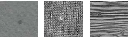
Figure 2. Examples of simple defect on the texture
On this type of defect, its density function has tendency to be a skew distribution, either to the left (dark gray level) or to the right (light gray level) depends on the gray level of the defected area. If the defected area is darker than the non-defected one, then the distribution will be skew to the left. Otherwise, it is skew to the right.
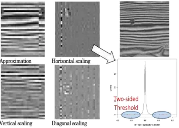
However, sometimes the defect is hard to detect directly from the original image, e.g. the defect on the wood (center image of Figure 2). The defected area will come to the surface if we use wavelet transform to the image. Wavelet transform is like Fourier Transform. Fourier Transform decomposes signal into sines and cosines, while wavelet decomposes signal into more general functions that follows several rules. Some examples of wavelet functions are Haar wavelets, Daubechies wavelets, Mexican hat. It is well known that wavelet is very powerful to detect “jump” on the pattern (Nason[11]). Therefore, before we proceed with finding the defect, we use wavelet transform as the first step of the procedure, and look for the most suitable space such that our method can perform well. Figure 3 and Figure 4 exhibit examples of finding a simple defect in the texture. At first, we transform the original image using wavelet transform. In Figure 3, the structure of the image is simple, the defect can be seen clearly as a spot in the image. In the approxi-mation space of the wavelet the spot is clearer than the other spaces, and the distribution of the gray level shows that the distribution is skew to the right. The correct threshold of the distribution will indicate, which area can be spotted as defect area, and which ones are not. While for the Figure 4, the structure of image in Figure 4 (that is wood) is more complex than the structure of image in Figure 3. Directly estimating the distribution of the gray level in Figure 4 will not make the defect area exhibit. However, using wavelet transform, we can see in the horizontal scaling, the defect part of the image is appeared. Additionally, the histogram of the gray level is stiff and it has two thresholds (in the left and right) for indicating the defect area.
Methods
The idea of this propose method is first, we trans-form the image into the wavelet space, since it is more robust for detecting the defect in the image (see Figure 4), and then using the kernel density we will calculate the density of the gray level of image. Kernel density is smoother than the histogram for estimating the density of the gray level. Finally, we used several methods for detecting the threshold for separating the defect spot to the not defect one.
In this section we will give a brief description of kernel density estimate, for detail explanation please refer to Wand and Jones [12]. Further, we will explore the threshold procedure for finding the defected area on the simple defect detection and at the end we present the result of this procedure.
Kernel Density Estimate (KDE)
Let be an i.i.d. sample drawn from a distribution with an unknown density ƒ. We are interested in estimating the shape of this function ƒ. Its kernel density estimator is;
̂ ∑ ∑ (1)
where is a kernel function and is the bandwidth.
Some properties of KDE: (1) To ensure should be symmetric and have a unique maximum at 0 and also ∫ is to take as probability density function (pdf). (2) To ensure that a kernel estimator has attractive mean squared error properties, it turns out to be important to choose so that ∫ , ∫ , ∫ ,
denotes for a kernel
Figure 3. The wavelet transform of the original image with the density estimate from the Approximation space.
Optimal Bandwidth
To get the optimal bandwidth we have to trade-off compromise between the bias and variance of the KDE. Fortunately, this trade-off comprise can be (MSE) of the estimator, since by definition:
̂ ̂ (2)
Take the integration of (2) then we get,
[∫( ̂ ) ] we get the Asymptotic MISE, i.e.
(6)
Finally, we take derivative of (6) with respect to and solve for the derivative equal to zero, then we get the optimal global bandwidth, i.e., the bandwidth will be the same for the whole function of estimate.
[
]
threshold, i.e. we assume that the probability of the defect gray level is greater than (or less than) for example 5%. The second one is automatic thres-holding using modified Otsu [13] methods and Hill estimation for measuring the tail of the distribution [14].Basically, before we define the threshold, we should know the shape of the gray level distribution, i.e., skew to the left, skew to the right or symmetry.
Simple Threshold
Depend on the shape of the gray level distribution, we can have either one-sided threshold (if the shape of distribution is skew to the left or right) or two-sided threshold (for symmetry distribution) (Figure 5). Let is the threshold, then if the shape of the for selecting optimal image threshold. Let the value of gray-level ranging from 0 to L-1, where L is the number of distinct gray level. Let the number of pixels with gray-level be and be the total number of pixels in a given image, then can be regarded as the probability of occurrence of gray-level and ∑ as the average of the entire gray-level. For a single thresholding, the pixels of an image are divided into two classes and where is the threshold value. The probabilities of the two classes are:
∑ and ∑ . The mean gray-level values of the two classes can be computed as
∑ ⁄ and ∑
⁄ (8)
Using discriminant analysis, Otsu [14] showed that the optimal threshold can be determined by maximizing the between-class variance, i.e.,
(9)
Where the between-class variance is defined as
(10) where the smaller the value of (low probability of occurrence), the larger the weight will be.
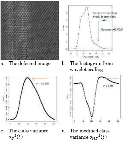
a. The defected image b. The histogram from wavelet scaling
c. The class variance
d. The modified class variance
Figure 6. An example of threshold points from defected texture using Otsu Method and Modified Otsu Method.
of two classes are ∫ ̂ and
∫ ̂ . While, the first moment of gray-level values of the two classes can be computed as;
∫ ̂ ⁄ and
∫ ̂ ⁄ , where ̂ is the estimate kernel density function.
A comparison of these two approaches is given in the Figure 6. The density of the defected image is right skew, the skewness measurement is positive (0.8358). It tells us that the defected area would belighter than the non-defected area, and it is matched to the image in Figure 6a, i.e., indeed the defected area is in nearly white color. Moreover, the expected threshold should be around 1.0 (the right tail of the distribution). We can see clearly in Figure 6c and 6d, that the threshold point suggested by is the reversed order statistics, is called the upper tail index. Hill [14], introduced an estimator
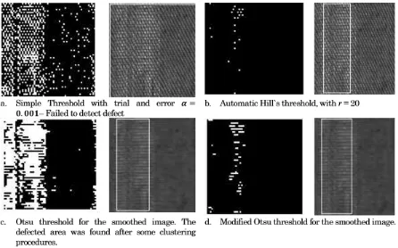
We compare three methods we presented above for a single image, which give different performances. First, we used a trial and error threshold. After several trial and errors, from large to small gray level probability, the trial could not detect the defected part of the texture (see Figure. 7a, for gray level probability, ). The defected pixels are scattered in the whole image.
Figure 8. Some result examples of detected defect using combination of three methods
1. Transfer the image into wavelet space, use the highest resolution: HH, GG, GH, HG; where H stands for smooth filter and G for bandpass filter (Nason [11]);
2. Measure the skewness of HH, if the skewness is zero then use the GG space;
3. Calculate the KDE of the chosen space; 4. Calculate the threshold:
a. Simple threshold: If the skewness > 0 then calculate the probability of right side of the distribution until it achieves the given . The stopping point is the threshold. Do the similar procedure for skewness < 0, for the left side of the distribution;
b. Hill estimator: use equation (15) and perform hypothesis test for exponential distribution. Stop until r in equation (15) differ the distribution from exponential. Calculate the probability under the r. If the probability is greater than then it is better to use simple threshold (4a) or modified Otsu method (4c) instead of this estimator;
c. Modified Otsu method: perform the modified Otsu method using (11);
5. Cluster the pixels which have gray level less than the threshold (for image which has left skew distribution) or greater than the threshold (for image which has right skew distribution); 6. Choose the most compact cluster which can be
performed from the three proposed methods; a. Defect detected in the
wavelet space
b. Defect detected in the original space
Notify the position by 4 outer points of the defect on the wavelet space and transfer those points to the original image. Mark the defect by white line on that position.
Conclusion
In this paper we transformed the original image into wavelet space and used kernel density for measuring the image histogram. We then applied three approaches for detecting the threshold points in the image density. The threshold points indicate the defect spot in the image. In the first approach, i.e. using simple threshold, we need to do some trial and error in determine the value of the alpha. While for the second and third approaches, i.e., modified Otsu and Hill estimator, the threshold can be detected automatically. We also proposed a procedure. The procedure will produces a rectilinear which cover the defect area (see Figure 7 and 8). The smallest the rectilinear can detect the defected area the better the performance of the proposed method. In this way of measurement, Hill estimator performs better than the other two proposed methods. which also will be elaborated in the future research.
Acknowledgment
manuscript for their comments and suggestions that greately improve the presentation of this paper.References
1. Peyré, G., Texture Synthesis with Grouplets, IEEE Transactions on Pattern Analysis and Machine Intelligence, 32(4), 2010, pp. 733-746. 2. Liu, L., and Fieguth, P., Texture Classification
from Random Features, IEEE Transactions on
Pattern Analysis and Machine Intelligence, 34(3), 2012, pp. 574-586.
3. Cavalin, P., Oliveira, L. S., Koerich, A. L., and Britto Jr, A.S., Wood Defect Detection using Grayscale Images and an Optimized Feature Set. IEEE Industrial Electronics, IECON 2006 -32nd Annual conference Proceeding, Paris 2006. 4. Yang Xue Zhi; Pang, G. K. H and Yung, N.H.C,
Fabric defect detection using adaptive wavelet,
Acoustics, Speech and Signal Processing,
Proceedings (ICASSP`01), Salt Lake city USA,
2001
5. Moahseri, B. B. M, Azadinia, S. and Mehbo-dniya, A New Voting Approach to Texture Defect Detection Based on Multiresolutional Decom-position, World Academy of Science, Engineering and Technology, 65, 2010, pp. 887-891.
6. Timm, F. and Barth, E., Non-parametric Texture Defect Detection using Weibull Features. Image Processing: Machine Vision Applications IV, 7877, Proceeding of SPIE. SPIE-IS& T. San Francisco, USA 2011.
7. Franke, J., and Halim, S., Wild Bootstrap Tests: Regression Models for Comparing Signal and Images, IEEE Signal Processing Magazine, July 2007, pp. 31-37.
8. Franke, J., and Halim, S., A Bootstrap Test for Comparing Images in Surface Inspection, pre-sented at DFG-Priority Program 1114 Technical Report 150.
9. Peng, Y., Wang, G. and Wang, H., User preferen-ces based software defect detection algorithms selection using MCDM, Information Sciences, 2012, 191, pp. 3-13.
10.Haindl, M., Texture Synthesis, CWI Quaterly, 1991, pp. 305-331.
11.Nason, G.P., Wavelet Methods in Statistics, Spri-nger, New York, 2008.
12.Wand, M.P and Jones, M.C; Kernel Smoothing, Chapman & Hall, 1995.New Jersey: Pearson Prentice Hall. 2005.
13.Ng Hui Fang, Automatic Thresholding for defect detection, Pattern Recognition Letters, 27(14), 2006,pp.1644-1649.
14.Hill, B. M., A Simple General Approach to Inference about the Tail of Distribution. Annals of Statistics, 3, 1975, pp. 1063-1174.