A SMOOTH DIFFUSION RATE MODEL OF WOOD DRYING:
A SIMULATION TOWARD MORE EFFICIENT PROCESS IN
INDUSTRY
Edi Cahyono1, Yudi Soeharyadi2, Mukhsar3
1,3) Faculty of Mathematics and Natural Sciences, Department of Mathematics, Universitas Haluoleo
Jl. Mayjen S. Parman, Kendari
Email: [email protected]; [email protected]
2) Faculty of Mathematics and Natural Sciences, Institut Teknologi Bandung
Jl. Ganesa 10, Bandung Email: [email protected]
ABSTRACT
In this paper we consider modeling of wood drying process in an industry. The process is conducted in a kiln oven. Mathematically, the drying inside the wood is considered as an initial and boundary value problem. The model is a diffusion equation where the diffusion rate depends on the moisture content of the wood. We investigate a smooth diffusion rate and we compare the model with real data from an industry. The model shows a good agreement with the real data. Moreover, the model shows a smoother process of drying, which is more desirable by the timber and lumber industries to improve their current methods of drying.
Keywords: modeling, wood drying, timber and lumber industries.
1. INTRODUCTION
A good drying process is very much of the interest of lumber and timber industries. This process may prevent the lumber from developing surface cracks and several other defects. It may reduce lumber weight by a factor two or more, which means a reduced transportation cost. It increases the lumber strength; nails, screws and glue hold better, paint and finishes adhere well. Dry lumber is a better thermal insulator than the wet one (see Budianto, 2003).
The moisture content (MC) of lumber is an important aspect on lumber drying. MC of lumber is defined as the ratio of the mass of water contained in the lumber to the mass of the lumber without water. MC of some fresh log cut from a tree may be above 100%. Industries dry lumbers to have MC around 6% to 20%.
To have good control on lumber drying, middle and large sizes timber industries dry lumber in (kiln) ovens. An oven and its schematic plot are presented in Figure 1, Cahyono et al. (2007). The moisture content of the lumber before entering the oven varies around 50% to 70%. In the drying process, the MC needs to be brought down to about 10%-15%. The drying process in the oven is done by controlling the Equilibrium Moisture Content (EMC), i.e. the air humidity in the oven. To make the process faster, the EMC should be lower, and vice versa. This can be achieved by automatically (computerized) controlling the heater, fan and ventilation all together.
Figure 1. An oven in industri and its schematic plot of a dry kiln oven
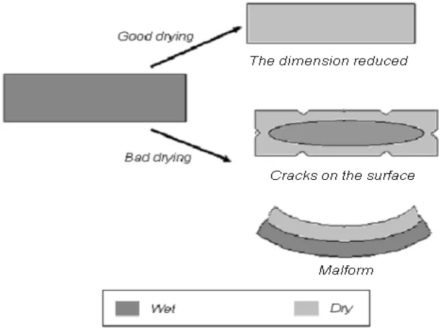
Figure 2. Drying affects a lumber to shrink, changes the form or develop cracks on the surface of the lumber
While drying process of the surface of lumber is directly controlled by setting the EMC, drying the inside part very much depends on the surface and also the type of lumber, hence it is not easily controlled. This paper discusses the drying process of the inside part of the lumber due to the given EMC, based on the research in Cahyono et al. (2007). Many previous researches are experimental tests or purely modeling and simulation, Omarsson (1999), Omarsson, et al. (1999), Omarsson, et al. (2000) dan Ormarsson, et al. (2003). In this paper we consider modeling, simulation and comparison with real data obtained in an industry. It is intended to understand the process better which will be a starting point for an efficent process.
approximation of the diffusion rate is presented in section 3. This approximation yields the so-called singularity. A better approximation by removing this singularity is the focus of this paper and discussed in section 4. In section 5 we present the performance of the proposed model by comparing with the real data from an industry. Finally we end this paper with conclusion and further research.
2. MATHEMATICAL MODEL
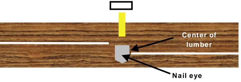
Although wood is a porous medium (Passard and Perre, 2001), we do not consider any models for porous media. Rather, we will consider macro scale model. Most of the discussion in this section is based on macro modeling presented in Beckum (2005). We consider a non-linear medium, e.g. wood and the water in it. In this macro-scale approximation we neglect the effects of the water particles and space between them and also the pores of the media.This approximation is motivated by the fact of wood drying process in industries. The water density i.e. the moisture content of wood is not measured at a ‘point’. Rather, it is measured in a small area which is thousands of the pore size of the wood, Cahyono (2005), Gubu and Cahyono (2005). Illustration of this measurement is given in Figure 3.
Figure 3. Measuring MC of lumber
For simplicity we will consider one-dimensional transfer, i.e. the geometry and the physics of two spatial variables are irrelevant. Cahyono and Solekan (2003) numerically showed that such simplicity can be applied to the heat transfer of a block of lumber where the length and the width are much larger than the thickness. Hence, the relevant physics and geometry are merely along the thickness of the lumber.
We write mass density (of water) at the point x∈ℜ (in the lumber) at the time t
by
ρ ρ
= ( , )x t . Let Ω = [x1, x2] be any closed interval inℜ. The total mass in Ω is given by∫
= 21 x
x dx
m ρ (1)
The rate of change of mass in Ω has the form
dx t t
m x
x
∫
∂ ∂ = ∂∂ 2
1
ρ (2)
Positive value of dm/dt means the total mass is increase and vice versa.
Let Φ(x1) and Φ(x2) be the flux at the point x1 and x2, respectively. The decrease of mass in Ω is given by
Ce nt e r of lum be r
2 1
(x ) ( )x
Φ − Φ (3)
Assuming the mass is conserved, the decrease of mass in Ω equals to the flux of mass leaving the point x1 dan x2
∫ =Φ −Φ = ∫ ∂∂Φ
∂ ∂ − 2
1
2
1
) ( )
( 2 1
x
x
x
x
dx x x
x dx t
ρ (4)
which is equivalent to
∫ ⎟ =
⎠ ⎞ ⎜
⎝ ⎛
∂Φ ∂ + ∂ ∂ 2
1
0
x
x
dx x t
ρ (5)
Assuming the integrant of (5) is continuous, we have
+ 0
t x
∂ρ ∂Φ =
∂ ∂ (6)
which is known as continuity equation.
The relation of the flux Φ(x, t) with state variable ρ(x, t) is based on the following reasoning. If at a given time t the state variable ρ(x, t) is not a constant function, then nature will flatten ρ by transfering quantity from places where the density is higher to the places where the density is lower. Hence, the flux Φ(x, t) is proportional and in opposite direction of the local steepness of
ρ(x, t). Mathematically, it is written
K x ∂ρ
Φ = − ⋅∂ (7)
For heat transfer (7) is Fourier’s law with thermal conductivity K; for spreading concentration (7) is Fick’s law with diffusion rate K. Hence, continuity equation has the form
K
t x x
∂ρ ∂= ⎛ ⋅∂ρ⎞ ⎜ ⎟
∂ ∂ ⎝ ∂ ⎠ (8)
For the case of wood which has neither nods nor annual rings, K does not depend on spatial variable but it is a function of ρ. Its mathematical expression, however, is still unknown. Cahyono (2005) approximates K by applying a step function, and Gubu and Cahyono (2005) approximate K
with a quasy-linear function. These approximations, however, yield discontinuity or unsmooth points on K.
3. CURRENT DIFFUSION RATE APPROXIMATION OF WOOD
We consider diffusion equation (8), where the diffusion rate is a function of the state variable. It has the form
(
( ))
tρ x K ρ xρ
∂ = ∂ ⋅∂ (9)
⎪
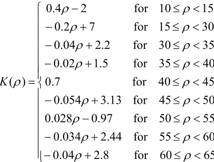
see Gubu and Cahyono (2005). Graphically, function (10) is plotted in Figure 4.
Notes:
Since
ρ
is comparison of mass of water and wood, then it has no dimension. K( )ρ
, however, does have dimension, i.e. M2 T -1. Through out this paper, M is in meters and T is in days.Figure 4. Piecewise linear approximation for diffusion rate
Observe that the approximation of K(ρ) with piecewise linear function yields point(s) where
K(ρ) is not differentiable. For the case of (10) these points are at ρ = 15, 30, 35, 40, 45, 50, 55, 60. On the other hand, equation (9) can be rewritten in the form
( )
2 24. REMOVING SINGULARITIES: SMOOTHING DIFFUSION RATE
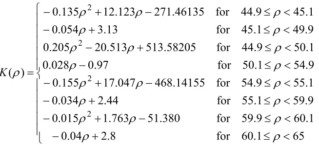
We will remove the singularity of the diffusion equation at the points where the piecewise linear diffusion rate is not smooth. On other word, we will smooth the diffusion rate on those points. This is illustrated in Figure 5. Applying piecewise linear function, the diffusion rate is given by ABC. It is not smooth at point B. We will smoothen this by considering a smooth curve APQC, by replacing the joint of two lines at point B with third order polynomial PQ. Detail of this smoothing process is as follows.
Figure 5. Smoothing piecewise linear function
Consider A(x1, y1), B(x2, y2) and C(x3, y3), where x1 < x2 < x3. The equation of line AB is given in the form
1( 2) 2
y=m x−x + y
and the equation of line AB is given in the form
2( 2) 2
y=m x−x + y
Hence, piecewise linear function for diffusion rate is given by
1 2 2 1 2
2 2 2 2 3
( ) ,
( ) ,
m x x y x x x
y
m x x y x x x
− + ≤ ≤
⎧
= ⎨ − + < ≤
⎩ (12)
in the interval [x1, x3]. Smoothing this function at point B, we consider point P(xp, yp) on line AB
and Q(xq, yq) on line BC. We will replace PBQ with third order polynomial PQ given by
3 2
( )
y= f x =ax +bx + +cx d (13)
We still need to seek the value of coefficients a, b, c, and d.
At point P(xp, yp) the value of f is yp. This gives a linear equation of a, b, c, and d
3 2
( p) p p p p
f x = y =ax +bx +cx +d (14)
The derivative of f at point P(xp, yp) is equal to the slope of AB, i.e, m1. Hence we have another linear equation of a, b, c, and d
2
1
'( p) 3 p 2 p
Similarly, at point Q(xq, yq) we have
ABC (12) with smooth piecewise polynomial function APQC in the form
1 2 2 1
a. Piecewise linear function (current diffusion rate)
b. Piecewise smooth polynomial function (proposed diffusion rate)
Figure 6. Current and proposed approximations of diffusion rate
Applying this ‘technique’, we smoothen piecewise linear function (12) with piecewise polynomial function in the form of (19). The details can be found in Cahyono et al. (2007). Comparing the linear function (12) with (19) graphically is not straight forward, except zooming in the region of unsmooth part of plot. This is shown in Figure 6.
⎪ example, the unsmooth point at ρ= 15. It has been removed by the definition of the piecewise function (19) in the interval [10, 29].
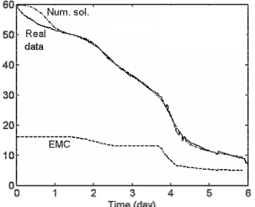
5. COMPARISON WITH REAL DATA
The state variable is the moisture content (MC) of wood. We consider lumber of durian wood (Durio zibethinus). The dimension is 5 cm x 40 cm x 250 cm and it is considered as a 1-D medium. We will compare the solution of our model with real data of MC of the lumber during the drying process. Note that the measurement of MC at center of the lumber, however, includes its surrounding area, but small, about hundreds or thousands of the pore size of wood. Hence, the MC does not refer only at a single point, rather an average quantity in its neighborhood. This technique is known as Representative Elementary Volume (REV), see Hornung (1997). In this paper we consider this by applying macro modeling. Equilibrium moisture content (EMC), which the humidity of the air inside the oven can be automatically controlled.
The numerical solution of the model (8) is computed numerically using a finite difference method. This method has been widely discussed in standard books such as Morton and Mayers (1996). For the numerical computation we use ∆x= 0.1, and the time step∆t=0.01. Let the
where the diffusivity K(Uij) is given by (19). The initial condition of the model is constant which is equal to the initial MC at the center of the lumber, the point where the MC is usually measured in industries. And, the boundary condition is equal to the EMC, where the MC of the lumber tends to be, mathematically it will achieve in infinite time.
Figure 7. Numerical solution and real data of MC and EMC
6. CONCLUSION AND FURTHER RESEARCH
We have proposed a new model of wood drying, a non-linear diffusion equation. The diffusion rate is a piecewise polynom function of the state variable. While we do not solve the model explicitly using analytical tools, we can solve it numerically. The numerical solution gives a remarkable match with industrial data, except in the beginning of the process. This may be caused by inaccurate initial condition.
The numerical result shows a smoother process of drying, which is desirable by the industries to improve their current methods of drying. The future research will be focused on the following. The first, we plan to look for an accurate initial condition. The second, developing model, which is an inverse problem, to find equilibrium moisture content (air humidity of the oven) to have a much more efficient drying process of wood. The third, we plan to improve the existing software to control the drying process based on the proposed model.
ACKNOWLEGDMENT
This research is supported by Ditjen Dikti, Depdiknas, Riset Fundamental contract no. 052/SP2H/PP/DP2M/III/2007. The first author thanks Ms Lily Koo, managing director of PT Harrison and Gil – Java, Semarang for the opportunity to do part of the research at PT HG – Java. The first author also thanks Mr Muh. Solikan of kiln division PT HG–Java for the fruitfull discussion. The authors would like to thank the anonymous referee for their valueable comments for the improvement of this paper.
REFERENCES
Beckum, F.van, 2005. “Macro and Micro Mathematical Modeling.” Prosiding Konferensi Nasional Matematika XII, Universitas Udayana, p. 9−23.
Cahyono, E., 2005. “Modeling of Wood Drying: A Step Function Approach to the Diffusivity.” Proceedings of the 2nd International Conference on Research and Education in Mathematics, Kuala Lumpur, Malaysia, p. 358–364.
Cahyono, E., and Solekan, 2003. “Model Perambatan Panas pada Proses Pengeringan Kayu.” Jurnal Matematika dan Komputer, Universitas Diponegoro, Vol. 6, No. 3, p. 118–127.
Cahyono, E., Soeharyadi, Y., and Mukhsar, 2007. Studi Numerik Proses Difusi pada Media Tak Linear: Aplikasi pada Proses Pengeringan Kayu, Laporan Penelitian, Lembaga Penelitian Universitas Haluoleo.
Gubu, La, and Cahyono, E., 2005. “A Quasi-Linear Diffusivity Approach for Diffusion Process of Lumber Drying.” Proceedings of the International Conference on Applied Mathematics, Bandung, Indonesia, p. 1002–1007.
Hornung, U., 1997. Homogenization and Porous Media, Editor: Hornung, U., Springer-Verlag, Berlin.
Morton, K.W., and Mayers, D.F., 1996. Numerical Solution of Partial Differential Equations, Cambridge University Press, Cambridge.
Omarsson, S., 1999. Numerical Analysis of Moisture Related Distortion in Sawn Timber, PhD Thesis, Dept. of Structural Mechanics, Chalmers University of Technology, Göteborg, Sweden.
Ormarsson, S., Cown, D., and Dahlblom, O., 2003. “Finite Element Simulations of Moisture Related Distortion in Laminated Timber Products of Norway Spruce and Radiata Pine.” 8th International IUFRO Wood Drying Conference, p. 27−33.
Omarsson, S., Dahlblom, O., and Peterson, H., 1999. “A Numerical Study of Shape Stability of Sawn Timber Subjected to Moisture Variation. Part 2: Simulation of Drying Board.” Wood Science and Technology, Vol. 33, p. 407−423.
Omarsson, S., Dahlblom, O., and Peterson, H., 2000. “A Numerical Study of Shape Stability of Sawn Timber Subjected to Moisture Variation. Part 3: Influence of Annual Ring Orientation.” Wood Science and Technology, Vol. 34, p. 207−219.