E
FFECTS
OF
DEM S
OURCE
AND
R
ESOLUTION
ON
WEPP H
YDROLOGIC
AND
E
ROSION
S
IMULATION
:
A C
ASE
S
TUDY
OF
T
WO
F
OREST
W
ATERSHEDS
IN
N
ORTHERN
I
DAHO
J. X. Zhang, J. Q. Wu, K. Chang, W. J. Elliot, S. Dun
ABSTRACT. The recent modification of the Water Erosion Prediction Project (WEPP) model has improved its applicability to
hydrology and erosion modeling in forest watersheds. To generate reliable topographic and hydrologic inputs for the WEPP model, carefully selecting digital elevation models (DEMs) with appropriate resolution and accuracy is essential because topography is a major factor controlling water erosion. Light detection and ranging (LIDAR) provides an alternative technology to photogrammetry for generating fine‐resolution and high‐quality DEMs. In this study, WEPP (v2006.201) was applied to hydrological and erosion simulation for two small forest watersheds in northern Idaho. Data on stream flow and total suspended solids (TSS) in these watersheds were collected and processed. A total of six DEMs from the National Elevation Dataset (NED), Shuttle Radar Topography Mission (SRTM), and LIDAR at three resolutions (30 m, 10 m, and 4m) were obtained and used to calculate topographic parameters as inputs to the WEPP model. WEPP‐simulated hydrologic and erosion results using the six DEMs were contrasted and then compared with field observations. For the study watersheds, DEMs with different resolutions and sources generated varied topographic and hydrologic attributes, which in turn led to significantly different erosion simulations. WEPP v2006.201 using the 10 m LIDAR DEM (vs. using other DEMs) produced a total amount of as well as seasonal patterns of watershed discharge and sediment yield that were closest to field observations.
Keywords. DEM, Forest watershed, GIS, LIDAR, Water erosion modeling, WEPP.
xcessive sedimentation in forest streams is one of the main concerns in forest management and water quality control (Luce, 1995). There is a need to ade‐ quately simulate and predict sedimentation from hillslopes to streams at the watershed scale in forested areas. However, simulation results can be greatly influenced by the topographic and hydrologic inputs (Renschler and Harbor, 2002). Numerous studies have shown that the reliability of the derived topographic and hydrologic attributes depends on the resolution and accuracy of the input digital elevation model (DEM), a common format for representing topogra‐ phy digitally (Jenson and Domingue, 1988; Chang and Tsai, 1991; Jenson, 1991; Florinsky, 1998; Gao, 1998; Schoorl et al., 2000; Claessens et al., 2005; Wechsler, 2007; Murphy et al., 2008). For example, Zhang and Montgomery (1994) re‐
Submitted for review in August 2008 as manuscript number SW 7657; approved for publication by the Soil & Water Division of ASABE in March 2009.
The authors are Jane Xinxin Zhang, Assistant Professor, Department of Geo/Physical Sciences, Fitchburg State College, Fitchburg, Massachusetts; Joan Q. Wu, ASABE Member Engineer, Associate Professor, Department of Biological Systems Engineering, Washington State University, Pullman, Washington; Kang‐Tsung Chang, Professor, Department of Tourism, Kainan University, Luzhu, Taoyuan, Taiwan; William J. Elliot, ASABE Member Engineer, Team Leader, USDA Forest Service, Rocky Mountain Research Station, Moscow, Idaho; and Shuhui Dun, Graduate Associate, Department of Biological Systems Engineering, Washington State University, Pullman, Washington. Corresponding author: Jane Xinxin Zhang, Department of Geo/Physical Sciences, Fitchburg State College, Fitchburg, MA 01420; phone: 978‐665‐3496; fax: 978‐665‐3081; e‐mail: [email protected].
ported that 10 m may be a proper resolution and a rational compromise between increasing resolution and data volume for simulating geomorphic and hydrological processes.
DEMs can vary in resolution and accuracy by the produc‐ tion method (Chang, 2006). The interval between elevation points determines the resolution of a DEM. The U.S. Geolog‐ ical Survey (USGS) offers 30 m and 10 m DEMs, which are the most common DEMs used in the U.S. Because of their limited availability, fine‐resolution DEMs (<10 m resolu‐ tion) have rarely been used for soil erosion simulation. A gap therefore exists in the literature for a systematic study of the effects of DEM resolution on soil erosion modeling for for‐ ested areas.
Recent developments in light detection and ranging (LIDAR) technology provide a new option for generating fine‐resolution DEMs (Hill et al., 2000; Liu, 2008; Murphy et al., 2008). LIDAR is an active remote sensing technology that uses light to determine the range between a target and a sensor. In an airborne LIDAR system, pulses of laser beam are emitted from an instrument mounted in an aircraft (Lee and Younan, 2003). The travel time of a pulse of light from the sensor to the reflecting surface and back is measured to determine the range to the surface. The horizontal coordi‐ nates (x,y) and elevation (z) of the reflective objects scanned by the laser beneath the flight path are obtained. The resultant measurements create a three‐dimensional cloud of points at irregular spacing, which can then be converted to a DEM.
The Water Erosion Prediction Project (WEPP) is a physi‐ cally based model for simulating erosion and sediment deliv‐ ery on hillslopes and watersheds (Flanagan and Nearing, 1995). WEPP uses climate, topography, soil, and manage‐
ment inputs to simulate infiltration, water balance, plant growth, residue decomposition, surface runoff, erosion, and sediment delivery over a range of time scales, including storm events, monthly, yearly, or long‐term annual average. WEPP was publicly released in 1995 and has undergone con‐ tinuous modifications since then to improve the model's abil‐ ity to simulate erosion in a variety of environmental conditions. Recent developments in WEPP, including modi‐ fications to the subsurface lateral flow routines, have im‐ proved the model's applicability in forest watershed modeling (Covert et al., 2005).
The geospatial interface for WEPP, GeoWEPP, was devel‐ oped to link the WEPP model with a GIS (geographic infor‐ mation system) and to utilize DEMs to generate the necessary topographic inputs for erosion modeling (Renschler et al., 2002; Renschler, 2003). The WEPP model uses a slope file to specify topographic elements, including slope length and gradient. GeoWEPP uses TOPAZ (Garbrecht and Martz, 1997) to automatically extract slope profiles from a DEM for WEPP applications. In the hydrology component of WEPP, slope is an input for deriving the maximum depression stor‐ age, i.e., the portion of rainfall excess held in storage due to micro‐variations in topography. Slope also directly affects surface runoff and subsurface lateral flow. In the erosion component of WEPP, topographic elements are used to calcu‐ late the shear stress acting on the soil, the friction coefficient, and the transport capacity of the flow. Thus, in WEPP ap‐ plications, DEM resolution and accuracy can influence hill‐ slope length, gradient, channel configuration, and channel slope in a watershed, which in turn affects the gross sediment yield at the watershed outlet as well as the spatial distribution of erosion along hillslopes and in channels. Many existing GeoWEPP applications have been based on 30 m USGS DEMs (Renschler and Harbor, 2002). The relatively coarse spatial resolution and low accuracy level of most existing DEM datasets has limited the WEPP model's simulation ca‐ pability.
The purpose of this study was to evaluate the effects of DEM resolution and accuracy on hydrology and water ero‐ sion simulation at a watershed scale using the improved WEPP model (v2006.201) under forest settings. Stream flow and sediment data in two small forest watersheds located on Moscow Mountain in Idaho were collected and processed. A total of six DEMs from three sources at three resolutions were evaluated for their ability in topographic parameterization for WEPP modeling. WEPP‐simulated long‐term runoff and erosion patterns in the study watersheds were examined.
M
ETHODOLOGYSTUDY AREA
The study area consists of two small forest watersheds, lo‐ cated at the southwest boundary of Moscow Mountain in La‐ tah County in northern Idaho. They cover a portion of the headwater area of the Paradise Creek watershed, which is part of the Palouse River hydrologic basin. Forested steep slopes and moderately steep rolling hills characterize the area. The elevation varies from 880 to 1300 m, and the slope ranges from 3% to 47%. The two watersheds were named wa‐ tersheds 5 and 6 corresponding to the respective monitoring sites, with watershed 5 forming the upstream section of wa‐ tershed 6. Watershed 5 (106 ha) contains the majority of steep
slopes, while watershed 6 (177 ha) includes most of the gentle slopes in the study area (Zhang et al. 2008).
The soil in the study area is a silt loam by the USDA soil textural classification (Hillel, 1982). It is derived from vol‐ canic ash, loess, and granitic residuum and is well drained. The bedrock of the watershed consists primarily of granite (Idaho DEQ, 1997).
Vegetation in the study area is coniferous forest dominated by Douglas fir and ponderosa pine. Much of the forested land in the Paradise Creek watershed had been subject to timber harvest. Since the landowner carried out a thinning operation as part of a healthy forest program in 1994, there has been minimal timber harvesting or related road construction. Rec‐ reational activities, such as hiking, mountain biking, and rec‐ reational vehicle riding, however, take place in the headwater area, which likely contribute to erosion and sedimentation of streams (Idaho DEQ, 1997; Crabtree, 2007).
Precipitation within the Paradise Creek watershed falls mainly in the winter (November to February) as either snow or a combination of rain and snow (Idaho DEQ, 1997). Dur‐ ing the spring months, snowpacks melt and cause prolonged high flows. Snowmelt coinciding with rainfall onto frozen soils typically generates high flows within the watershed. In the headwaters, Paradise Creek is intermittent, running for several months from the spring thaw until May or June. In the summer, flow stops, reducing the stream to a dry creek bed (Idaho DEQ, 1997).
DEM DATAAND PREPARATION
LIDAR data over the study area were acquired through Horizons, Inc. (Rapid City, S.D.), a LIDAR service company. The progressive morphological filter algorithm (Zhang et al., 2003) was applied to generate DEMs from the LIDAR data. The algorithm is commonly used for extracting ground points from LIDAR point clouds (Liu, 2008). The algorithm sepa‐ rates ground from nonground points, mostly vegetation in this case, by gradually increasing the window size of the filter and using elevation difference thresholds based on terrain characteristics of the study area. Ground points extracted from the LIDAR data were interpolated by ordinary kriging to create 4 m, 10 m, and 30 m DEMs.
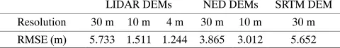
Table 1. Root mean square error (RMSE) of the six DEMs from three sources at three resolutions used in the study.
LIDAR DEMs NED DEMs SRTM DEM
Resolution 30 m 10 m 4 m 30 m 10 m 30 m
RMSE (m) 5.733 1.511 1.244 3.865 3.012 5.652
GPS points in and around the study area. A total of 18 GPS points were logged using Trimble TSC1 Asset Surveyor and differentially corrected by the GPS Pathfinder Office soft‐ ware. The accuracy of the GPS system was tested to be 0.826m vertically and 0.704 m horizontally. Point elevations at the 18 GPS locations were extracted from each of the six DEMs by bilinear interpolation, and their RMSE values were calculated using these point elevations against GPS measure‐ ments. The LIDAR 4 m and 10 m DEMs have the least RMSE, and the LIDAR and SRTM 30 m DEMs have the larg‐ est errors (table 1). The two NED DEMs, similar in accuracy, have the moderate level of RMSE.
FIELD OBSERVATIONS
Stream flow and total suspended solids (TSS) for wa‐ tersheds 5 and 6 were measured by the Latah Soil and Water Conservation District and Idaho Soil Conservation Commis‐ sion at the monitoring sites on Paradise Creek every two weeks starting March 1999. The observation lasted until De‐ cember 1999 with 18 records for watershed 5, and until June 2002 with 65 records for watershed 6. Daily values of wa‐ tershed discharge and sediment yield were calculated from these records through linear interpolation. Annual values were determined by integration, and their averages were ob‐ tained. For watershed 5, the average annual watershed dis‐ charge was 1.39 × 10⁵ m3 and the sediment yield was 1.38t.
For watershed 6, the average annual watershed discharge was 4.07 × 10⁵ m3 and the sediment yield was 4.55 t. These field
measurements were used in this study as the basis for compar‐ ison with simulated data.
WEPP APPLICATIONTO WATERSHED 5
WEPP was first applied to watershed 5, the upstream wa‐ tershed. Input files describing the watershed's climate, soil, management, and topography were prepared. Since the mod‐ el domain was small with relatively homogeneous condi‐ tions, we used one climate file for the watershed and two sets of soil and management files, one for hillslopes and the other for channels.
Existing climate data for the study area, including daily precipitation and maximum and minimum temperatures, were downloaded from the U.S. National Climatic Data Cen‐ ter (NCDC) Local Weather Observation Station Record web‐ site (NCDC, 2005). The data were observed at the University of Idaho station, Moscow, Idaho, the closest weather station to the study area (9 km to the southwest). The WEPP climate file includes additional inputs such as storm characteristics (duration, time to peak, and peak intensity), solar radiation, wind data (speed and direction), and humidity (dewpoint temperature). The random climate generator CLIGEN (Nicks et al., 1995), an auxiliary program of WEPP, was used to generate the other required weather data while preserving the observed temperature and precipitation data. A total of 30 years of climate input were prepared for 1973 to 2002, which covers the observation period of 1999 to 2002. Compared to the 30‐year average precipitation of 684 mm, annual precipi‐
tation of 695, 583, 588, and 590 mm for the observation peri‐ od represented average to relatively dry conditions.
The management input was based on the default data in WEPP for a 20‐year‐old forest (Elliot and Hall, 1997) with 100% ground cover, consistent with the observed conditions in the study area. The soil input was mainly based on the default values provided by WEPP for a silt loam in a 20‐year‐old forest. The default soil depth of 400 mm, shallower than reported by the Soil Conservation Service (USDA, 1981), was adopted as it better resembled the field conditions. Several soil parameters were adjusted in order to attain adequate water balance for the study area. The bedrock hydraulic conductivity was set to 3.6 × 10⁻⁶ mm/h based on the physical characteristics of granite
(Domennico and Schwartz, 1998) underneath the study area. The effective surface hydraulic conductivity was set to 105 mm/ h with a soil anisotropy ratio of 50. The initial saturation level of the soil profile was changed from the default value of 0.5 to 0.7 to properly represent actual soil water conditions in winter. The rock contents in the soil input were increased from 20% to 40% for hillslopes, and to 50% for channels.
These adjustments, carried out separately in a preliminary assessment, yielded a water balance, including stream flow and ET, that were compatible with field observations and literature values.
The topographic inputs for both hillslope profiles and channels were derived from each of the six DEMs through the TOPAZ application in GeoWEPP. TOPAZ uses a breaching‐ filling operation for removal of depressions and pits and the D8 algorithm (using the deterministic eight‐neighbor method to simulate flow across a land surface) for determining the drainage direction (USDA, 2008). For this study, the critical source area (CSA) was set to 10 ha and the minimum source channel length (MSCL) to 100 m in TOPAZ to make the derived channel networks and watershed structures agree with USGS digital raster graphic (DRG) maps.
The majority of the channel parameters were kept to the default values; however, for rocky channels in the study area, several parameters were adjusted. The channel erodibility was decreased from 6 × 10⁻⁴ to 5 × 10⁻⁴ s/m to mimic more
stable channels. The default depths to non‐erodible layer in mid‐channel and along the side of the channel were decreased from 0.5 to 0.04 m and from 0.1 to 0.03 m, respectively, in accord with field observations.
The aforementioned parameter adjustments were not carried out in favor of any DEMs but were for all six DEMs. The six DEMs generally responded in the same trend of increasing or decreasing watershed discharge and sediment yield simulations to the adjusted parameters. Subsequently, a 30‐year continuous WEPP simulation for watershed 5 was performed using the adjusted soil and channel inputs, together with the weather input based on observed precipitation and temperature plus additional weather variables generated by CLIGEN.
WEPP APPLICATIONTO WATERSHED 6
STATISTICAL ANALYSES
WEPP‐simulated average annual watershed discharge and sediment yield for the 30‐year period (1973 to 2002) for the two watersheds were compared to the observed values. Observation records for both watershed 5 (March to December 1999) and watershed 6 (March 1999 to June 2002) were rather short. Comparison of average annual values was preferred for two main reasons. First, a 30‐year simulation period is generally adequate for estimating long‐term average erosion potential (Elliot et al., 1999). Second, the climatic input for the WEPP simulations was a combination of observed and CLIGEN‐generated weather data, rendering detailed year‐by‐year comparison inappropriate. The nine‐ month observed watershed discharge and sediment yield data for watershed 5 were interpolated (March to December) and extrapolated (January to March) to one‐year values, and the 39‐month observed data for watershed 6 were averaged to yearly values.
Analysis of variance (ANOVA) tests were performed to determine the effects of DEM resolution with two levels (coarse, 30 m; and fine, 10 m and 4 m), DEM source with three levels (NED, SRTM, and LIDAR), and the interaction of resolution and source with six levels.
Visual examination of WEPP‐simulated watershed discharge and sediment yield from the six DEMs versus field observations suggested the 10 m LIDAR DEM to be the most reliable topographic input source (Zhang et al., 2008) (detailed discussion included in the next section). Hence, all subsequent statistical analyses on the impacts of topographic features on WEPP simulations were conducted using the 10m LIDAR DEM.
Correlation analyses (a = 0.05) were carried out to
examine how climatic and topographic factors may affect watershed discharge and sediment yield simulations. The four rainfall parameters evaluated were annual precipitation, annual precipitation of previous year, annual average rainfall intensity, and annual average rainfall peak intensity, with the first two climatic parameters being observed and the last two computed based on the CLIGEN‐generated storm characteristics data. The annual average rainfall intensity was calculated as the mean of the average rainfall intensity of all individual storms in a year, and the annual average rainfall peak intensity was the mean of the rainfall peak intensity of all the events in that year.
A correlation analysis (a = 0.05) was also made to assess
the relationships among annual watershed discharge, subsurface lateral flow, ET, sediment yield, and major topographic factors of hillslope length and gradient. The hillslope aspect, ranging from 0° (due north) to 360°, was categorized into four principal directions and four diagonal directions. An ANOVA was performed to evaluate the same hydrologic and erosion outputs as affected by hillslope aspect.
R
ESULTSANDD
ISCUSSIONSGeoWEPP‐determined watershed configurations for watersheds 5 and 6 are presented in Zhang et al. (2008). In general, coarse DEMs (30 m) resulted in blocky watershed boundaries as well as unsmooth hillslopes and stream networks for both watersheds. Fine‐resolution DEMs (10 m and 4 m), especially the two LIDAR DEMs, exhibited
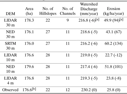
Table 2. GeoWEPP‐determined watershed configuration and WEPP‐simulated average watershed
discharge and erosion for watershed 5.
DEM
112.3 18 7 215.3 (65) 156.7 (1109)
LIDAR [a] Percent relative errors are in shown in parentheses.
[b] Topographic parameters, including watershed area, number of
hillslopes, and number of channels, were derived using TOPAZ in GeoWEPP. As a comparison, these topographic parameters derived from ArcGIS 9 using LIDAR 4 m are included here.
substantially improved representations of general topographic features. Further analysis of slope statistics revealed that, as DEM resolution degraded, an averaging of elevations and slopes occurred, which is consistent with the findings of Chang and Tsai (1991), Florinsky (1998), and Gao (1998). WEPP‐simulated watershed discharge and sediment yield using the six DEMs for watersheds 5 and 6, together with the field observations, are presented in tables 2 and 3.
WATERSHED 5
The different DEMs resulted in slightly different watershed areas, and considerably different numbers of hillslopes and channels. All DEMs led to overestimated watershed discharge and sediment yield except the 10 m
Table 3. GeoWEPP‐determined watershed configuration and WEPP‐simulated average watershed
discharge and erosion for watershed 6.
DEM [a] Percent relative errors are in shown in parentheses.
[b] Topographic parameters, including watershed area, number of
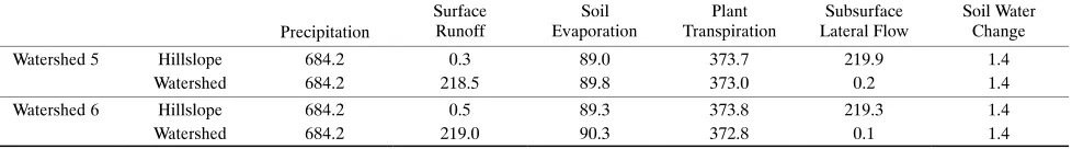
Table 4. Thirty‐year average annual water balance (mm) for watersheds 5 and 6 from WEPP simulations using the 10 m LIDAR DEM
Precipitation
Surface Runoff
Soil Evaporation
Plant Transpiration
Subsurface Lateral Flow
Soil Water Change
Watershed 5 Hillslope 684.2 0.3 89.0 373.7 219.9 1.4
Watershed 684.2 218.5 89.8 373.0 0.2 1.4
Watershed 6 Hillslope 684.2 0.5 89.3 373.8 219.3 1.4
Watershed 684.2 219.0 90.3 372.8 0.1 1.4
NED, which resulted in an underestimated sediment yield. The simulated watershed discharges were 65% to 69% greater than the observed value. The simulated sediment yields were 9% to 1109% higher than the observation, with the exception of a 3% underestimate using the 10 m NED. All three 30 m DEMs led to overestimations of sediment yield by more than 50% with the 30 m LIDAR and SRTM DEMs overpredicting by 300% and 1100%, respectively. The 10 m and 4 m LIDAR DEMs improved the model performance greatly. The simulation using the 10 m NED DEM generated an overestimate of watershed discharge but an underestimate of erosion.
WEPP‐simulated average annual water balance from the 10 m LIDAR DEM, on both hillslope and watershed levels and weighted by area, is presented in table 4. Surface runoff originating from hillslopes is minimal. Soil evaporation and plant transpiration account for 13% and 55%, respectively, totaling 68% of annual precipitation. Subsurface lateral flow amounts to 32%. WEPP v2006.201 assumes that all subsurface lateral flows from hillslopes discharge into the stream channel, as reflected in the water balance for watershed 5. The slightly higher evaporation and lower plant transpiration on the watershed level than on the hillslope level is due to the inclusion of channels with high open‐water evaporation and lack of plant transpiration.
WATERSHED 6
Excluding the 30 m LIDAR, all DEMs produced similar watershed area and similar numbers of hillslopes and channels for watershed 6. Compared to the smaller and topographically more complex watershed 5, watershed 6 appears to have a more consistent spatial delineation.
WEPP‐simulated watershed discharges using the six DEMs were agreeable with, though consistently lower (~6%) than, the field observation. This outcome was in contrast with the results for watershed 5, for which all watershed discharge simulations were overestimates. A likely reason could be that this version of WEPP does not model groundwater base flow and, consequently, deep percolation on hillslopes in headwater areas is not further routed to downstream channels. The overestimate of runoff for the upstream watershed 5 might result from the use of an underestimate of the hydraulic conductivity for the bedrock, which could in turn lead to an underestimate of deep percolation. Consequently, the underestimate of runoff for the downstream watershed 6 could be due to the lack of base flow.
Four DEMs generated overestimates of sediment yield, and two (10 m and 4 m LIDAR) produced underestimates. The 30 m SRTM led to the poorest simulation of erosion (upward 130%). The other two 30 m DEMs (LIDAR and NED) produced similar erosion simulations (roughly 70% to 90% overestimate). Although the 10 m NED yielded a rather satisfactory erosion simulation for watershed 5, it had a highly disagreeable result (over 100%) for watershed 6.
Sediment discharge was measured with an ISCO sampler located at the downstream end of a relatively flat reach of channel, carrying low amounts of sediment. Although this was ideal for measuring flow rates, there may have been sediment deposition in this reach, reducing the amount of sediment collected. The 10 m and 4 m LIDAR DEMs generated better simulations than all the other four DEMs and had consistent underestimations of watershed discharge and sediment yield. Overall, the simulations of watershed discharge and sediment yield were much closer to the observed data for watershed 6 than for watershed 5.
WEPP‐simulated average annual water balance for watershed 6 is similar to that for watershed 5 (table 4). The increase in evaporation and stream flow is a result of increase in stream network density. The area ratio of channel to watershed is 0.19% for watershed 5 and 0.26% for water-shed 6. That the WEPP‐simulated stream flow accounts for more than 30% of precipitation is consistent with the field observation.
STATISTICAL ANALYSES
The ANOVA results indicated that, at a significance level of 0.05, DEM resolution and source did not have a significant effect on simulated watershed discharge; however, the DEM source had a significant effect on the simulated erosion (p = 0.02).
The correlation analyses indicated significant influence of all the annual climatic parameters on the simulated watershed discharges for watersheds 5 and 6 at a significance level of 0.05 and 0.01 (table 5). The high correlation between the simulated watershed discharges for the two watersheds reflected their spatial relationship. The relatively low correlation between climatic parameters for the previous and present year can be attributed to the high interannual variation in precipitation (SD = 120 mm). The correlation results appeared reasonable and revealed that a number of climatic parameters worked together to induce overland flow, alter soil water, and generate total watershed discharge. No significant correlation was detected between the climatic factors and the sediment yield simulations for either watershed. The study area is forested with surface cover throughout seasons. Consequently, minimal surface runoff is generated, and watershed discharge is primarily composed of subsurface lateral flow (table 4). The simulated watershed discharge was substantially influenced by climatic factors, and the simulated water erosion was mainly driven by hillslope surface runoff and channel flow.
Table 5. Correlation among climatic parameters and WEPP‐simulated annual watershed discharge and sediment yield using 10 m LIDAR DEM.[a]
Annual
[a] ** = significant at α = 0.05; p‐values of the correlation coefficients are shown in parentheses.
Table 6. Correlation between topographic parameters and WEPP‐simulated annual water balance and sediment yield for watershed 5 using 10 m LIDAR DEM.[a]
Hillslope
[a] ** = significant at α = 0.05; p‐values of the correlation coefficients are shown in parentheses.
Table 7. Correlation between topographic parameters and WEPP‐simulated water balance and sediment yield for watershed 6 using 10 m LIDAR DEM.[a]
Hillslope
[a] ** = significant at α = 0.05; p‐values of the correlation coefficients are shown in parentheses.
amounts of lateral flow, which in turn reduces surface runoff (Crabtree, 2007). Consequently, hillslope gradient negatively influences simulated erosion, which is particularly true for watershed 5. The simulated ET was not affected by hillslope length and gradient, as expected.
The impact of hillslope aspect on ET was significant for both watersheds 5 and 6. The impact of hillslope aspect was
also significant on surface runoff and subsurface lateral flow for watershed 5, and on lateral flow for watershed 6. Erosion was not related to hillslope aspect.
Table 6 shows that erosion is inversely proportional to lateral flow, although not significantly at a = 0.05, whereas
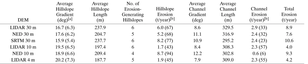
Table 8. WEPP‐simulated spatial distribution of erosion as affected by topographic factors for watershed 5.
[a] Standard deviations of hillslope gradients are shown in parentheses.
[b]Ratios (%) of hillslope (or channel) erosion to total erosion are shown in parentheses.
Table 9. WEPP‐simulated spatial distribution of erosion as affected by topographic factors for watershed 6.
DEM
[a] Standard deviations of hillslope gradients are shown in parentheses.
[b] Ratios (%) of hillslope (or channel) erosion to total erosion are shown in parentheses.
effects of lateral flow reducing surface erosion than in watershed 6 (tables 8 and 9). At these low levels of erosion with few storm events causing surface runoff, even a small difference in hydrologic conditions can lead to a large variation in simulated erosion rates. The flatter, shorter hillslopes delineated for watershed 6 may have been less impacted by lateral flow processes. Another unexpected result in table 7, which may also be attributed to the aforementioned reasons, is that erosion is negatively correlated with runoff, once again not significantly at a =
0.05. Additional factors complicating the interrelationship among simulated hydrologic and erosion results include the masking of topographic impacts on hydrologic and erosion processes by weather patterns, and the characteristics of snowmelt runoff. For the study watersheds, most snowmelt runoff was simulated to occur early in the season at low rates from saturated soils. Only rarely was a large runoff event simulated, generally linked to a rain event on a melting snowpack. Hence, it is reasonable that the majority of runoff generated no erosion, but a very few high‐intensity runoff events generated large amounts of erosion. The simulated total runoff from these large events, however, is unlikely to be as large as the simulated total runoff from the low‐intensity snowmelt events, which are more common.
EROSION SIMULATIONSAS IMPACTEDBY DEMS
Tables 8 and 9 show erosion simulations as affected by topographic factors, i.e., average hillslope and channel gradients and lengths extracted by GeoWEPP from the six DEMs for watersheds 5 and 6. Generally, coarser DEMs generated leveler topography but higher sediment yield simulations than finer DEMs. This result may be counterintuitive; however, DEM‐derived terrain factors affected erosion simulations in a complex manner. Average slope gradient is only one of the many factors that affect erosion. The different DEMs resulted in substantially
different hillslope and channel systems, and a combination of all the topographic attributes work together to impact WEPP‐ simulated gross sediment yield at the watershed outlet and the partition of erosion between hillslopes and channels.
As an example, the 30 m SRTM DEM delineated the flattest and the smoothest (with lowest standard deviation of slope gradient) hillslopes for both watersheds, but it resulted in much higher sediment yield than other DEMs, likely for the following reasons. First, it delineated the longest hillslope length in watershed 5 and the second longest in watershed 6. Longer hillslopes tend to generate higher runoff rates (tables6 and 7), thus increasing the erosion potential. Second, the SRTM DEM produced the highest number of erosion‐generating hillslopes for both watersheds and, in turn, resulted in substantially higher hillslope erosion. Hillslope erosion was the major form of erosion for both watersheds (63% of total erosion for watershed 5 and 77% for watershed 6). Third, the SRTM DEM delineated relatively steep channel slopes for both watersheds. Steep channel slopes increase stream flow velocity, and thus channel erosion. On the other hand, the SRTM DEM generated the second shortest average channel length in watershed 5, and the shortest in watershed 6. Therefore, the impacts of steeper channel slope and shorter channel length would somewhat be offset in influencing channel erosion, but both channel characteristics (steeper and shorter) would likely increase the delivery of sediment eroded from the hillslopes.
Channel erosion was the major form for both watersheds (roughly 60% of total erosion) for this DEM. Additionally, lower sediment transport and delivery could have resulted from more accurate depiction of the flatter toes of hillslopes using finer DEMs (Zhang et al., 2008). In general, the standard deviation of slope gradient decreases as DEM resolution becomes coarser. Finer‐resolution DEMs depict more details of terrain, both steep and gradual slopes, which results in greater variation of slope gradient among hillslopes.
The 10 m and 4 m LIDAR DEMs resulted in consistent simulation of the spatial partition of erosion for the two watersheds. Among the other four DEMs, the 10 m NED DEM simulated dominant channel erosion for watershed 5 (79% of total erosion) and dominant hillslope erosion for watershed 6 (94% of total erosion).
Overall, most erosion simulations were overestimates except those from using the 10 m and 4 m LIDAR DEMs for watershed 6. Erosion simulations were poorer for water-shed 5 than for waterwater-shed 6. Topographically, the smaller watershed 5 has steeper terrain. Hence, it is crucial to have accurate topographic inputs to realistically represent such complexity. Many forests are in mountainous areas with steep slopes and complex terrain. Our results show that carefully selecting appropriate DEMs with proper accuracy and resolution is critical to modeling hydrologic and erosion processes in forested areas.
LONG‐TERM WATERSHED DISCHARGEAND SEDIMENT YIELD
Results from the 30‐year (1973 to 2002) WEPP simulation using the 10 m LIDAR DEM for watersheds 5 and 6 revealed similar seasonal patterns of runoff and erosion. Most runoff events were simulated to occur in winter and spring with peak flows corresponding to snowmelt in spring, consistent with field observations. The simulated erosion events were driven by runoff events, as shown in figure 1 for watershed 6. The years 1977, 1993, 1994, and 2001 had no erosion events simulated because of the low stream flows.
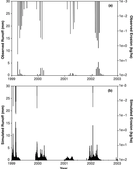
Comparison of WEPP‐simulated and field‐observed watershed runoff and erosion for 1999 to 2003 showed good agreement in seasonal pattern (fig. 2). Note that field observation prior to March 1999 was not available. WEPP tended to overpredict peak runoff for high flow conditions (Conroy et al., 2006). WEPP simulated substantially fewer
Year
1973 1976 1979 1982 1985 1988 1991 1994 1997 2000 2003
Runoff (mm)
0 20 40 60 80
Erosion (kg/ha)
1e-3
1e-2
1e-1
1e+0
1e+1
1e+2
1e+3
1e+4
1e+5
1e+6
1e+7
Figure 1. WEPP‐simulated 30‐year watershed runoff (bottom) and erosion (top) events for watershed 6 using the 10 m LIDAR DEM (erosion rate in log scale).
erosion events. The simulated runoff events corresponded well with larger runoff events, but generally had lower erosion rates (nearly one magnitude lower), compared to field observations. Figure 2 shows that WEPP simulated more days with runoff than observed because the remote weirs were set to record large runoff events only, to conserve battery power and save sample bottles for large events. We have not shown the interpolated flow values between observations in figure 2. WEPP simulations had higher peak flow rates than observed, similar to Conroy et al. (2006), although the total runoff from watershed 6 was less than observed (table 3). One of the reasons may be that WEPP (v2006.201) generated all of the watershed runoff from surface runoff and subsurface lateral flow, while the observed runoff also included influences from groundwater base flow in this steep watershed. There appears to be a justification for adding algorithms for groundwater base flow to the WEPP model to moderate surface runoff and peak channel flows without decreasing total runoff.
Other reasons may include the uncertainty associated with: (1) the weather data, which were from the closest weather station located 9 km away from the study area, (2)CLIGEN‐generated missing weather data, and (3) field‐ observed data that were interpolated and extrapolated (see, e.g., Harmel and Smith, 2007). Temme et al. (2006) discussed the uncertainty in simulation of water erosion due to uncertainty in filling DEM sinks. We recognize that uncertainty in the DEM data used in this study may have impacted our WEPP simulations.
WEPP‐simulated annual watershed runoff and erosion in comparison with yearly precipitation for watersheds 5 and 6
1999 2000 2001 2002 2003
Observed Runoff (mm)
0 5 10 15 20 25 30
Observed Erosion (kg/ha)
1e -3
1e -2
1e -1
1e+0
1e+1
1e+2
Year
1999 2000 2001 2002 2003
Simulated Runoff (mm)
0 5 10 15 20 25 30
Simulated Erosion (kg/ha)
1e -3
1e -2
1e -1
1e+0
1e+1
1e+2
(a)
(b)
Year
1973 1977 1981 1985 1989 1993 1997 2001
Precipitation and Runoff (mm)
0 200 400 600 800 1000
Precipitation (mm) Simulated runoff (mm) Simulated erosion rate (kg/ha)
Year
Erosion Rate (kg/ha)
1e-1 1e+0 1e+1 1e+2 1e+3 1e+4
Runoff (mm)
100 150 200 250 300 350 400 450 500
Count
0 2 4 6 8 10
Simulated Observed
Runoff (mm)
100 200 300 400 500
Erosion Rate (kg/ha)
0 100 200 300
Count
0.1 1 10 100
Simulated Observed
Erosion Rate (kg/ha)
0 100 200 300 400
(a) (b)
(c) (d)
(e) (f)
1999 Obs.
1999-2002 Obs. 1999
Obs.
1999 Obs.
2000 Obs. 2001
Obs. 2002Obs.
1973 1977 1981 1985 1989 1993 1997 2001
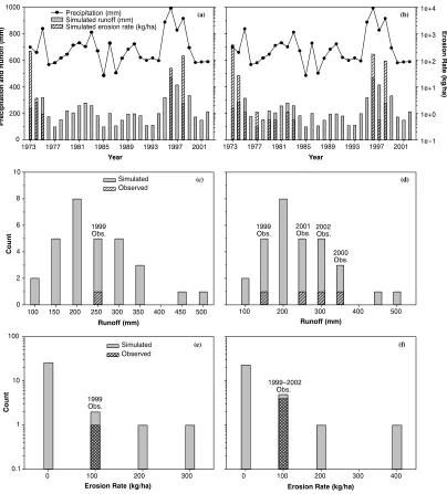
Figure 3. WEPP‐simulated annual watershed runoff and erosion with (a and b) annual precipitation and (c to f) histograms. The left graphs are for watershed 5 and the right graphs for watershed 6.
are shown in figures 3a and 3b. Annual runoff strongly correlated with annual precipitation, as also indicated by the correlation analysis (table 5). Erosion was simulated for five years for the smaller watershed 5, and eleven years for the larger watershed 6. For both watersheds, major erosion occurred in the two wettest years of 1996 and 1998. Additionally, high erosion was also simulated to occur in the first year as a result of the channel erosion algorithm in current WEPP. This outcome was likely linked to the oversimulation of peak runoff rates (Conroy et al., 2006), which in turn resulted in large channel flow rates, and a large initial erosion rate, before the non‐erodible layer was reached in the channel.
Histograms of WEPP‐simulated annual watershed runoff (figs. 3c and 3d) for the two watersheds are identical. The single observation record for watershed 5 and the four records for watershed 6 generally fall in the middle range of simulated annual watershed runoff. The histograms of WEPP‐simulated annual erosion for the two watersheds (figs. 3e and 3f) are different. The larger watershed 6 can
generate higher annual erosion (400 kg/ha) compared to the upstream watershed 5 (300 kg/ha). For both watersheds, simulated annual erosion most frequently fell into the zero and 100 kg/ha category, whereas the field observations tended to fall into the 100 kg/ha category.
S
UMMARYANDC
ONCLUSIONSRunoff simulations using different DEMs did not differ substantially due to the typical hydrologic characteristics of forested areas, where subsurface lateral flow is predominant. Erosion simulations from the 10 m LIDAR DEM were most consistent and agreeable with field observations. The coarser, 30 m DEMs generated smoother topography and produced poor estimates of erosion, with the 30 m SRTM DEM overpredicting sediment yield by 10 fold. The 10 m NED DEM gave inconsistent erosion simulations. The 4 m LIDAR DEM did not improve the model simulations over the 10 m LIDAR DEM.
For the study watersheds, WEPP v2006.201 using the 10m LIDAR DEM (vs. using other DEMs) produced a total amount of as well as seasonal patterns of watershed discharge and sediment yield that were closest to field observations. The current WEPP version tended to simulate relatively high channel erosion in the initial period of simulation. Future efforts can be devoted to examining the channel erosion algorithms in WEPP, to improving snow hydrology processes, and to incorporating the ability of quantifying groundwater base flow into WEPP to properly simulate runoff from steep forested watersheds.
ACKNOWLEDGEMENTS
We thank Erin Brooks and Bill Dansart for providing us the field‐observed runoff and sediment yield data, Jim Frankenberger for his valuable advice and suggestions on using the GeoWEPP interface, and Sue Miller, Andy Hudak, and Jeff Evans for their help with processing the GPS and LIDAR data. We are grateful to ASABE Associate Editor Dr. R. Munoz‐Carpena and three anonymous reviewers for their valuable and constructive comments that greatly helped to improve the rigor and clarity of the manuscript.
R
EFERENCESChang, K. T. 2006. Introduction to Geographic Information Systems. 4th ed. New York, N.Y.: McGraw‐Hill.
Chang, K. T., and B. W. Tsai. 1991. The effect of DEM resolution on slope and aspect mapping. Cartogr. Geogr. Info. Sci. 18(1): 69‐77.
Claessens, L., G. B. M. Heuvelink, J. M. Schoorl, and A. Veldkamp. 2005. DEM resolution effects on shallow landslide hazard and soil redistribution modeling. Earth Surf. Process. Landforms
30(4): 461‐477.
Conroy, W. J., R. H. Hotchkiss, and W. J. Elliot. 2006. A coupled upland‐erosion and instream hydrodynamic‐sediment transport model for evaluating sediment transport in forested watersheds.
Trans. ASABE 49(6): 1713‐1722.
Covert, S. A., P. R. Robichaud, W. J. Elliot, and T. E. Link. 2005. Evaluation of runoff prediction from WEPP‐based erosion models for harvested and burned forest watersheds. Trans. ASABE 48(3): 1091‐1100.
Crabtree, B. E. 2007. Variable source area hydrology modeling with the Water Erosion Prediction Project (WEPP) model. MS thesis. Moscow, Idaho: University of Idaho.
Domennico, P. A., and F. W. Schwartz. 1998. Physical and Chemical Hydrogeology, 39‐40. 2nd ed. New York, N.Y.: John Wiley and Sons.
Elliot, W. J., and D. E. Hall. 1997. Water Erosion Prediction Project (WEPP) forest applications. Gen. Tech. Rep. INT‐GTR‐365. Ogden, Utah: USDA Forest Service, Rocky Mountain Research Station.
Elliot, W. J., D. E. Hall, and D. L. Scheele. 1999. WEPP:Road, WEPP interface for predicting forest road runoff, erosion, and
sediment delivery. Technical documentation. Moscow, Idaho: USDA Forest Service, Rocky Mountain Research Station, and San Dimas, Cal.: San Dimas Technology Development Center. Available at: http://forest.moscowfsl.wsu.edu/fswepp/docs/ wepproaddoc.html. Accessed 2 July 2005.
Flanagan, D. C., and M. A. Nearing. 1995. USDA Water Erosion Prediction Project (WEPP): Hillslope Profile and Watershed Model Documentation. NSERL Rep. 10. West Lafayette, Ind.: USDS‐ARS National Soil Erosion Research Laboratory. Florinsky, I. V. 1998. Accuracy of local topographic variables
derived from digital elevation models. Intl. J. Geogr. Info. Sci.
12(1): 47‐61.
Gao, J. 1998. Impact of sampling intervals on the reliability of topographic variables mapped from grid DEMs at a micro‐scale.
Intl. J. Geogr. Info. Sci. 12(8): 875‐890.
Garbrecht, J., and L. W. Martz. 1997. TOPAZ: An automated digital landscape analysis tool for topographic evaluation, drainage identification, watershed segmentation, and subcatchment parameterization: TOPAZ overview. ARS Pub. No. GRL 97‐2. El Reno, Okla.: USDA‐ARS Grazinglands Research Laboratory. Harmel, R. D., and P. K. Smith. 2007. Consideration of
measurement uncertainty in the evaluation of goodness‐of‐fit in hydrologic and water quality modeling. J. Hydrol. 337(3‐4): 326‐336.
Hill, J. M., L. A., Graham, and R. J. Henry. 2000. Wide‐area topographic mapping and applications using airborne light detection and ranging (LIDAR) technology. Photogramm. Eng. Remote Sensing 66(8): 908‐914.
Hillel, D. 1982. Introduction to Soil Physics. San Diego, Cal.: Academic Press.
Idaho DEQ. 1997. Paradise Creek TMDL‐water body assessment and total maximum daily load. Lewiston, Idaho: Idaho Division of Environmental Quality, Lewiston Regional Office.
Jenson, S. K. 1991. Application of hydrologic information automatically extracted from digital elevation models. Hydrol. Proc. 5(1): 31‐44.
Jenson, S. K., and J. O. Domingue. 1988. Extracting topographic structure from digital elevation data for geographic information system analysis. Photogramm. Eng. Remote Sensing 54(11): 1593‐1600.
Lee, H. S., and N. H. Younan. 2003. DTM extraction of LIDAR returns via adaptive processing. IEEE Trans. Geosci. Remote Sensing 41(9): 2063‐2069.
Liu, X. 2008. Airborne LiDAR for DEM generation: Some critical issues. Prog. Phys. Geogr. 32(1): 31‐49.
Luce, C. H. 1995. Forests and wetlands. In Environmental Hydrology, 253‐284. A. D. Ward and W. J. Elliot, eds. Boca Raton, Fla.: CRC Lewis.
Murphy, P. N. C., J. Ogilvie, F. R. Meng, and P. Arp. 2008. Stream network modeling using lidar and photogrammetric digital elevation models: A comparison and field verification. Hydrol. Proc. 22(12): 1747‐1754.
NCDC. 2005. Asheville N.C.: U.S. Department of Commerce, National Climatic Data Center. Available at:
www.ncdc.noaa.gov/oa/ncdc.html. Accessed 22 January 2005. Nicks, A. D., L. J. Lane, and G. A. Gander. 1995. Chapter 2:
Weather generator. In USDA Water Erosion Prediction Project: Hillslope Profile and Watershed Model Documentation. D. C. Flanagan and M. A. Nearing, eds. NSERL Rep. 10. West Lafayette, Ind.: USDA‐ARS National Soil Erosion Research Laboratory.
Renschler, C. S. 2003. Designing geo‐spatial interfaces to scale process models: The GeoWEPP approach. Hydrol. Proc. 17(5): 1005‐1017.
Renschler, C. S., and J. Harbor. 2002. Soil erosion assessment tools from point to regional scales: The role of geomorphologists in land management research and implementation. Geomorphology
Renschler, C. S., D. C. Flanagan, B. A. Engel, and J. R.
Frankenberger. 2002. GeoWEPP: The geospatial interface to the Water Erosion Prediction Project. ASAE Paper No. 022171. St. Joseph, Mich.: ASAE.
Schoorl, J. M., M. P. W. Sonneveld, and A. Veldkamp. 2000. Three‐dimensional landscape process modeling: The effect of DEM resolution. Earth Surf. Process. Landforms 25(9): 1025‐1034.
Temme, A. J. A. M., J. M. Schoorl, and A. Veldkamp. 2006. Algorithm for dealing with depressions in dynamic landscape evolution models. Comput. Geosci. 32(4): 452‐461.
USDA. 1981. Soil survey of Latah County Area, Idaho. Washington, D.C.: USDA Soil Conservation Service.
USDA. 2008. Research/TOPAZ‐General Information. Washington, D.C.: USDA‐ARS. Available at: www.ars.usda.gov/Research/ docs.htm?docid=7835#lt. Accessed 30 March 2009.
Wechsler, S. P. 2007. Uncertainties associated with digital elevation models for hydrologic applications: A review. Hydrol. Earth Syst. Sci. 11(4): 1481‐1500.
Zhang, J. X., K. T. Chang, and J. Q. Wu. 2008. Effects of DEM resolution and source on soil erosion modelling: A case study using the WEPP model. Intl. J. Geogr. Info. Sci. 22(8): 925‐942. Zhang, K., S. C. Chen, D. Whitman, M. L. Shyu, J. Yan, and C.
Zhang. 2003. A progressive morphological filter for removing nonground measurement from airborne LIDAR data. IEEE Trans. Geosci. Remote Sensing 41(4): 872‐882.
Zhang, W., and D. R. Montgomery. 1994. Digital elevation model grid size, landscape representation, and hydrologic simulations.
![Table 7. Correlation between topographic parameters and WEPP‐simulated waterbalance and sediment yield for watershed 6 using 10 m LIDAR DEM.[a]](https://thumb-ap.123doks.com/thumbv2/123dok/2116755.1609430/6.612.55.556.481.627/table-correlation-topographic-parameters-simulated-waterbalance-sediment-watershed.webp)