Exploratory Research on Developing Hadoop-based Data Analytics Tools

Exploratory Research on Developing Hadoop-based

Data Analytics Tools

Henry Novianus Palit, Lily Puspa Dewi, Andreas Handojo, Kenny Basuki, Mikiavonty Endrawati Mirabel Department of Informatics

Petra Christian University Surabaya, Indonesia

hnpalit@petra.ac.id, lily@petra.ac.id, handojo@petra.ac.id, kennybasuki@gmail.com, mikiavonty@gmail.com

Abstract—As we crossed past the millennium mark, slowly but steadily we were flooded by (digital) data from virtually everywhere. The challenges of big data demand new methods, techniques, and paradigms for processing data in a fast and scalable fashion. Most enterprises today need to employ data analysis technologies to remain competitive and profitable. Alas, the adoption of big data analysis technologies in Indonesia is still in its infancy, even in the academic sector. To encourage more adoptions of big data technologies, this study explored the development of Hadoop-based data analytics tools. Two case studies were used in the exploration. One is to showcase the performance comparison between Hadoop and DBMS, whereas the other is between Hadoop and a statistical analysis tool. Results clearly demonstrate that Hadoop is superior in processing a large data size. We also derive some recommendations to tune Hadoop optimally.

Keywords—Hadoop; MapReduce framework; big data analysis; performance comparison; Hadoop tuning.

I. INTRODUCTION

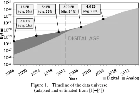
As we entered the new millennium in 2000, we were also subconsciously entering the digital age, where the amount of digital data has exceeded that of the analog. Fig. 1 shows the growth of the data universe as well as the digital data shares for the past three decades.

In 1986, the amount of data in the world was estimated around 3 Exabytes (1 Exa = 1018), in which only 1% of those

were in digital formats. With the proliferation of the Internet and its applications, the amount of digital data increased faster than the analog counterpart and reached 25% of the data universe in 2000. The turn of the century saw the staggeringly rapid growth of the digital data, owing to the spread of the 3rd Platform of computing (i.e., mobile, hi-def devices, soc-med, cloud) [4]. Within two years, the digital data had equaled, and then surpassed, the analog; the year 2002 marked the beginning of the Digital Age.

Meanwhile, the total data stored in the world had reached 54 Exabytes at the turn of the century, and increased nearly 6-fold to 309 Exabytes in 2007, and further increased 15 times to 4.6 Zettabytes (1 Zetta = 1021) in 2014. By large and

far, today’s data universe is about 20 Zettabytes, in which the

digital data has taken the lion’s share (i.e., more than 99%). In addition, IDC had forecasted that the global datasphere would continue to grow to 44 and 163 Zettabytes in 2020 and 2025, respectively [3]–[4], as can be seen also in Fig. 1.

Indeed, we are flooded by data from virtually everywhere (i.e., from the apps in our computers, our mobile apps, sensors in our vehicles, our home and office appliances, and many other sources). According to IDC, now approximately there are 15 billion devices connected to the Internet [5]. The figure is predicted to double to 30 billion by 2020, and then almost triple to 80 billion by 2025. It clearly demonstrates the phenomenal growth of IoT (Internet of Things) that also contributes to the data explosion.

However, not all data are essential to businesses and consumers. About 10% of the current data are critical to our daily lives and require real-time processing. But that portion of data is still very large, roughly equivalent to 2 Zettabytes. By 2025, nearly 20% of the global data are life-critical [4]. Think about autonomous cars, remote monitoring patient devices, self-healing power grid, and other advances in the near future. New methods and techniques, commonly called Big Data analytics, are used to promptly analyze those data.

In Indonesia, the adoption of big data analysis technologies is still in its infancy. Nevertheless, IDC Indonesia reported that 70% of business enterprises interviewed in 2004 planned to pilot a big data project within that year, making it the second most coveted technology after mobile applications [6]. Retailers, e-commerce, telecomm, logistics, and financial companies are those which have lots of data and are poised to gain benefits from analyzing them.

Figure 1. Timeline of the data universe (adapted and estimated from [1]–[4])

By

te

s

Year Digital Analog 1015

1016

1017

1018

1019

1020

1021

1022

1023

1024

4.6 ZB (dig. 98%) 309 EB

(dig. 94%) 54 EB

(dig. 25%) 16 EB

(dig. 3%)

2.6 EB (dig. 1%)

DIGITAL AGE

Government agencies also have started to employ big data analysis [7]–[9] to gain insights and make policies. Other lines of industry, even those small and medium enterprises (SMEs), will inevitably follow suit or lose out in the competition.

Clearly, the demand for data analytics talents is very high. MGI estimated that, while data science graduates could increase by 7% per year, the projected demand might grow 12% annually, which would lead to a shortage of 250,000 data scientists [10]. Similarly, there will be high demands for business translators (bridging data scientists and practical business applications) and visualization experts (bringing complex data to live visualization for decision makers).

As an academic institution, we are inherently responsible to offset the imbalance between the high demand and low supply of data-savvy graduates. Alas, only a number of tertiary institutions in Indonesia offer compulsory subjects related to big data analysis. Even in our institution, it is still an elective subject.

This research is trying to explore Hadoop MapReduce, an open source framework for writing applications that can process very large data. People are saying that big data is expensive and only big businesses can afford it. To debunk that myth, we deployed Hadoop not on sophisticated servers, but on off-the-shelf desktops in one of our common computer laboratories. We have two-pronged goals of doing this exploratory work:

1. To gain knowledge and understanding of developing Hadoop applications, and in the same time, train our students to master the skills;

2. To embolden more interests from academics and industries in Indonesia to adopt and leverage big data analysis technologies, and show them that it is possible to have that capability at a low cost.

The rest of the discussion is arranged in this order. Section 2 gives the overview of Big Data and Hadoop, as well as discusses some related works. Section 3 presents the case studies for our exploration with Hadoop and details case problems to be addressed in this study. Experimental results are presented and discussed in Section 4. Finally, we wrap up the manuscript with the conclusion and future works in Section 5.

II. TECHNOLOGY OVERVIEW AND RELATED WORKS

This section is begun with a brief overview of Big Data. After that, the original MapReduce and GFS are described, and are immediately followed by their clones in the Hadoop project. In the last subsection, some related works are discussed and compared with our work.

A. Big Data

The term “big data” had been included in OED [11] since 2013. It is unclear who really coined the term. Sociologist Charles Tilly [12] was probably the first to use the term, but the context of which was different from our current understanding. The next publication to use the term was authored by Cox and Ellsworth [13]; they asserted that the

“big data” problem taxes the computer’s capacity. However,

Mashey [14], then a Chief Scientist at SGI, was largely credited as the first to champion the concept of “big data”.

Gartner’s Laney [15] indicated the three dimensions of data management challenge: Volume, Velocity, and Variety (often popularized as 3Vs). Data volume refers to the enormous amount of data collected. Data velocity deals with the fast pace of data generated, whereas data variety deals with the many sources, types, and forms of data. Some people have added more Vs to the original 3Vs. IBM, for example, added another V for Veracity [16], pertaining to the data uncertainty or trustworthiness.

Apart from all the lingos and jargons, “big data” really

demand a drastic change in the way we capture, store, manage, process, and analyze them. The traditional approach of executing a data analytic application on a single machine is no longer working, since data grow much faster than the computer’s capacity and capability can cope with. A scalable approach is required to address the big data challenges. The next subsection introduces one of the scalable platforms, i.e., MapReduce.

B. MapReduce and GFS

MapReduce is a programming model initially proposed by Google [17]. It is a simple yet powerful interface that enables parallel and distributed computations. Using this programming model, a developer needs to create two functions: Map and Reduce. The Map function accepts an input key/value pair and generates a set of interim key/value pairs. The MapReduce library automatically groups all interim values having the same interim key, before passing them to the Reduce function. The Reduce function takes each interim key and its associated set of interim values, and generates output result(s), which is typically a single value, but may also be a set of values. Conceptually the MapReduce model can be illustrated as follows:

In the Map function, the domain of the input k1/v1 pair is

often different from that of the interim k2/v2 pairs. By

contrast, the domain of the interim k2/set(v2) pair in the Reduce function is usually the same as that of the output

set(v3). The MR_Combiner function is inherent in the MapReduce model; it does the grouping mentioned in the earlier paragraph. Note that the MapReduce library can spawn multiple Map and Reduce processes on a cluster of machines; hence, the data processing can be executed in a parallel and distributed fashion. Furthermore, it is scalable since the developer can increase or decrease the number of processes as needed.

To support the programming model, Google proposed a scalable distributed file system, called Google File System (GFS) [18]. A GFS cluster comprises a single master and multiple chunkservers. Files are divided into fixed-size chunks, which are stored in the chunkservers with replication (the default is 3 replicas per chunk). The chunk replication serves two purposes: a) maximize data reliability and availability, and b) optimize network bandwidth utilization.

Map(k1, v1)  set(k2, v2)

MR_Combiner(k2, v2)  set(k2, set(v2))

Each chunk is assigned a unique handle. A GFS client application needs to implement the file system API to read and write data. Clients interact with the master for metadata operations and with the chunkservers for all data-bearing communication.

C. Hadoop MapReduce and HDFS

Inspired by the published GFS and MapReduce papers, Doug Cutting and Mike Cafarella developed a similar platform while working on a web crawler project called

Nutch. Later on, the platform’s development was spun off as

an independent open-source project called Hadoop [19]. Thus, Hadoop is essentially the open-source counterpart of

Google’s MapReduce framework. Hadoop is developed using Java; by contrast, Google’s MapReduce is in C++. Similar to the original version, the core of Hadoop is Hadoop MapReduce (distributed computing) and HDFS / Hadoop Distributed File System (storage system) [20]. There is no change to the MapReduce paradigm in Hadoop. Likewise, HDFS only changes the service component terminology from “master” to “NameNode”, and “chunkservers” to

“DataNodes”.

With the introduction of YARN (Yet Another Resource Negotiator) as the resource manager in the second generation of Hadoop, MapReduce is no longer the only distributed computing framework in Hadoop ecosystem. As shown in Fig. 2, Spark and Tez are examples of other distributed computing frameworks that may run on top of HDFS and HBase (i.e., Hadoop’s NoSQL Database).

D. Related Works on Hadoop

Manikandan and Ravi [21] listed various analytics tools related to Hadoop, such as Hive, Pig, Avro, Mahout, etc. They also explained the MapReduce’s components and how they work in big data analysis.

Hadoop is not a mature product; it still has some issues to be addressed. Besides, Hadoop has a lot of parameters that can be tuned differently in different scenarios to achieve optimal performance.

Huang et al. [22] evaluated Hadoop’s MapReduce mechanisms and identified potential areas that can be optimized. Such examples are the single point of failure, the problem of small size but large number of files, and some parameter tuning issues. They further explored Hadoop’s deployment in cloud computing.

Vellaipandiyan and Srikrishnan [23] also experimented with Hadoop in cloud computing. They observed the CPU and memory utilization, as well as the execution time, while running Hadoop jobs with different BlockSize+SplitSize

settings. They concluded that it is preferable to run Hadoop with higher than default BlockSize when the data being processed are very large.

The many configurable parameters in Hadoop beg a recommendation for tuning it optimally. Our work will

partially address the quest for Hadoop’s optimal settings.

Since BlockSize is an important parameter in Hadoop’s HDFS, it will be one of the parameters that we investigate. Other important parameters for optimal execution are the numbers of mappers and reducers.

Hadoop is capable of processing different datasources (files) in parallel owing to its multiple DataNodes, yet each DataNode processes data in a sequential manner. Saldhi et al. [24] proposed parallel processing in each DataNode by leveraging the multicore processor available on the underlying machine. Employing the proposed analytics platform for solving a business use case, they managed to plot profit trends of different products quickly and efficiently.

Another case of solving a big data analytics problem with Hadoop was demonstrated by Nandimath et al. [25]. Employing a collage of technologies such as Hadoop and NoSQL database in Amazon Web Services, they calculated the average ratings, total recommendations, total votes, and such, of interesting locations the users shared in a social networking application.

Although Hadoop’s MapReduce and relational DBMS

take different approaches in processing data, they may be used to solve similar data retrieval problems. The comparison between the two has not been fully addressed in previous works. We will investigate this comparison in our work. Another overlapping data processing is between

Hadoop’s MapReduce and statistical analysis tools (like MATLAB, SPSS, or R). It interests us to compare them too in this study.

III. DATA ANALYSIS CASE STUDIES

To try out Hadoop’s capability, we used two case studies. The first case study was the book circulation data of our university’s library. Simple analyses are regularly performed on the data with the help of a DBMS. We tried to imitate the same analyses on Hadoop. The second case study was an online user profile dataset retrieved from Yahoo Research. We conducted simple correlation analyses on some of the user attributes. The following subsections further explain these two case studies.

A. Book Circulation Data

The data comprised 6 master tables and 1 circulation history table. We received all the tables in CSV (comma-separated values) format. We applied preprocessing on the master tables to remove headings, quotes, carriage-return characters (note: Linux just recognizes the line-feed character as the end of line), and more importantly, to add missing records to ensure referential integrity. Details of the preprocessed master tables are listed in Table I.

The circulation history was collected from January 2011 to June 2014. In total, there were 182,426 records (about 19,853.75 KB file size) that we received. We were told that

in July 2013 there was a change in the application used for borrowing and returning books, and that change affected the way the book circulations were recorded. Before the change, one record would completely store the information from when a book was borrowed, how many times it was renewed, until when it was returned. But after the change, each transaction (either a borrowing, renewing, or returning) would be stored as a record; thus, multiple records would be generated for a borrowing-(renewing-)returning cycle.

TABLE I. MASTER TABLES FOR BOOK CIRCULATION DATA

Table Name Content No. Recs Size (KB) m_department Prefix codes and names of

the uni’s departments.

21 0.48

m_book_type Types of book collections maintained by the library.

35 1.88

m_av_type Types of audio-visual collections maintained by the library.

26 0.91

m_location Sections of the library where the collections are stored.

29 1.25

m_title Titles of collections (books and audio-visual materials) and related details.

129,591 31,244.58

m_item Collection items (including multiple copies of an item) and related details.

159,307 32,211.14

Those two versions of circulation history had to be processed differently. Hence, we split it into two tables: one for the stand-alone records and the other for the inter-related records. The former had 106,693 records (about 13,657.24 KB file size), whilst the latter had 75,733 records (about 9,139.77 KB file size).

Queries involving multiple tables were executed to reveal the following information:

A1.Number of borrowing transactions per audio-visual collection type.

A2.Number of borrowing transactions per book collection type.

A3.Number of borrowing transactions per collection title.

A4.Number of borrowing transactions per location (i.e., library section).

A5.Number of borrowing transactions per department. In all cases, the number of borrowing transactions also includes the number of renewing transactions. For an example, if a book is borrowed by a student and then renewed twice before being returned by the student, then the resulting number of borrowing transactions is three.

B. Online User Profile Dataset

This dataset was retrieved with permission from Yahoo Webscope Program (belonging to Yahoo Research) [26].

The dataset could be found in the “Graph and Social Data” catalog with id G7 and was titled “Yahoo! Property and Instant Messenger Data use for a Sample of Users”. The

compressed size of this dataset is 4.3 GB, and when it is uncompressed, the total size is about 13 GB.

The dataset was collected from October 1 to October 28, 2007. It comprised 31 tab-delimited text files, which could be categorized into 9 types, as shown in Table II.

TABLE II. FILE TYPES OF YAHOO’S DATASET

File Type Content

User data (YD1) General Yahoo! user profiles that had been anonymized.

IM use (YD2) Instant messaging activities.

PC network use Number of accesses using PC (non-mobile). Country via IP lookup Countries from which the accesses came. PC front page, mail,

search use

Accesses to front page, mail, and search using PC.

PC other property use Accesses to other Yahoo! properties (i.e., weather, news, finance, sports, and Flickr) using PC.

Mobile web use (YD3)

Accesses to Yahoo! mobile web pages.

Yahoo! Go use Accesses to Yahoo! Go pages. Mobile web Flickr

errata

Errata to Yahoo! mobile Flickr accesses.

Not all files were used in the study. Only some attributes from user data, IM use, and mobile web use, which are respectively marked as YD1, YD2, and YD3 in Table II, were selected and analyzed. The following statistical analyses were investigated:

B1. Correlation between age (in YD1) and communication frequency (in YD2)

B2. Correlation between gender (in YD1) and different mobile web page views (in YD3)

IV. RESULTS AND DISCUSSION

We experimented with the Hadoop implementations of the required data analyses. The experimental results for both case studies are presented and discussed in this section.

A. Book Circulation Data

Cases A1–A5 above can be addressed in SQL. For an example, the following SQL query is for addressing case A1:

That query involves three master tables (i.e., m_item, m_title, and m_av_type), and the two transaction tables (i.e., t_circ_hist_standalone and t_circ_hist_interrelated). Similar

SELECT d.k245h AS av, SUM(c_number) AS c_number FROM ((SELECT k999a, 1+SUM(c_renew) AS c_number FROM t_circ_hist_standalone

GROUP BY k999a) UNION ALL

(SELECT k999a, 1+MAX(c_renew) AS c_number FROM t_circ_hist_interrelated

GROUP BY id_member, k999a, date_borrowed) ) AS a,

m_item b, m_title c, m_av_type d

WHERE a.k999a = b.k999a AND b.no_cat = c.no_cat AND c.av_type = d.av_type

GROUP BY av

SQL queries can also be developed for cases A2–A5, in each of which 3 to 5 tables are merged by union and join operations.

For each query case, we developed an associated application in Hadoop. Select operations were implemented in the mapper, whilst union and join operations were in the reducer. Afterwards, we compared the query executions in a MySQL database and in Hadoop. Observed parameters were CPU utilization, RAM (memory) utilization, and execution time. The Hadoop applications were executed on a single desktop (acting as both the NameNode and DataNode) with a 4-core CPU and 16-GB RAM.

Table III contrasts the execution results (averaged from a number of trials) in (MySQL) DBMS and Hadoop. Clearly, the query executions in DBMS are faster (27–214 times) and more efficient (4–19 folds on CPU utilization and 10–12 folds on RAM utilization) than those in Hadoop. This is understandable since the amount of data is considered small for Hadoop.

TABLE III. EXECUTION COMPARISON BETWEEN DBMS&HADOOP FOR ORIGINAL DATA

Case CPU Util. (%) RAM Util. (MB) Exec. Time (secs) DBMS Hadoop DBMS Hadoop DBMS Hadoop A1 80.13 361.30 174.67 1935.23 0.98 101.34 A2 43.03 388.07 174.60 1908.13 0.60 79.10 A3 85.40 316.27 175.85 1702.24 2.98 80.99 A4 20.90 390.00 175.06 2028.81 0.37 79.34 A5 23.17 319.20 174.94 2026.57 0.41 58.58

TABLE IV. EXECUTION COMPARISON BETWEEN DBMS&HADOOP FOR MULTIPLIED DATA

Case CPU Util. (%) RAM Util. (MB) Exec. Time (secs) DBMS Hadoop DBMS Hadoop DBMS Hadoop A1 100.50 402.43 312.80 3199.65 4241.35 1670.57 A2 100.80 402.37 218.61 3147.96 3739.29 1637.47 A3 100.17 403.07 254.68 3320.71 3719.59 1641.31 A4 100.50 403.17 247.16 3263.10 3612.47 1638.88 A5 129.27 402.83 291.22 3182.76 925.38 1673.55

To truly see Hadoop’s capability, we multiplied the circulation history (both, the stand-alone and inter-related versions) 425 times and slightly changed the values of the primary keys to maintain their uniqueness. By doing this, we boosted the total transaction data size from 22.26 MB to 9.24 GB. As can be seen in Table IV, the results are quite the opposite from those shown previously in Table III. Query executions in DBMS are still more efficient (3–4 folds on CPU utilization and 10–14 folds on RAM utilization); of course, the resource usage of a single core execution is much less than that of multiple cores’ counterpart. However, the resulting execution times in Hadoop are just 39–45% of those in DBMS, except for case A5 where the DBMS’s

execution is faster than the Hadoop’s counterpart. The query for case A5 needs an additional process to retrieve a substring of id_member (if its length is exactly 8 characters) to determine the student member’s department. The Hadoop application for case A5 may require a more optimized algorithm to handle the additional process. Based on the

overall results, it can be concluded that data analyses using Hadoop are beneficial when the data size is very large, involving multiple records, fields, and/or tables (i.e., files).

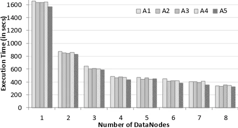
We further evaluated the impact of adding more DataNodes to the execution of Hadoop applications. We found that the execution times are reduced as the number of DataNodes increases. As the number of DataNodes is increased gradually from 1 to 4 nodes, the execution time is improved 22–48%. Afterwards, adding more DataNodes only improves the execution time marginally (i.e., <10%). Fig. 3 depicts the impact of adding more DataNodes.

We also executed the Hadoop applications with different HDFS BlockSizes. Our finding is slightly different from

Vellaipandiyan and Srikrishnan’s [23]. We found that the BlockSize of 128 MB, which is the default setting in HDFS, is the most optimal BlockSize, yielding the best execution times. It was also observed that the most optimal execution occurs when the file size is close to (but still less than) the BlockSize.

B. Online User Profile Dataset

For case B1, Pearson’s correlation [27] was employed to determine whether age and communication frequency were related. The spread of data can be seen in Fig. 4. As it can be

noticed, some data tell us that the user’s age is above 100

years old. The users might deliberately conceal their true age by giving any number. We had no means to correct the data. However, since our objective is just to explore Hadoop’s

Figure 4. Plotting users based on age and communication frequency

0 200 400 600 800 1000 1200 1400 1600

1 2 3 4 5 6 7 8

E

x

ec

u

ti

o

n

T

ime

(i

n

s

ec

s)

Number of DataNodes

A1 A2 A3 A4 A5

capability, we proceeded to analyze the data without modification.

We developed Hadoop applications to accomplish

Pearson’s correlation. From YD1, the user id, gender, and age were retrieved in a mapper process. Separately, from YD2, the user id and communication frequency were generated in another mapper process. The two generated data were then joined in a reducer process. The Person’s correlation coefficient was evaluated on the joined data (between age and communication frequency) by another MapReduce job. The yielded result is r = −0.001 and ρ < 0.001, which indicates no correlation between age and communication frequency.

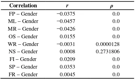
Case B2 involve two sets of attributes with different nature. Mobile web page views are multiple (comprising 9 different pages) regular scores, whereas gender is a two-value score (i.e., 1 for man and −1 for woman). The former were retrieved from YD3, whilst the latter was from YD1. We calculated the correlation coefficients between gender and each of the mobile web pages. Since gender is dichotomous or binomial, then the point-biserial correlation [27] was employed to determine its correlation with the mobile web page views.

The same mapper that retrieved user id, gender, and age from YD1 was again employed. The nine mobile web pages (then provided by Yahoo) are Front Page (FP), Mail (ML), Messenger (MR), One Search (OS), Weather (WR), News (NS), Finance (FI), Sports (SP), and Flickr (FR). We developed another mapper that could retrieve those data from YD3, indexed by the user id. The two sets of data were joined in a reducer process. Another MapReduce job was created to calculate the point-biserial correlation. The yielded correlation results can be observed in Table V. All results indicate very weak correlations between age and mobile web page views. Nevertheless, we can see modest tendencies that men access Sports more than women, while women prefer to access Mail, Messenger, and Front Pages more.

TABLE V. RESULTS OF CORRELATION EVALUATION BETWEEN AGE AND MOBILE WEB PAGE VIEWS

Correlation r ρ

FP – Gender −0.0375 0.0 ML – Gender −0.0457 0.0 MR – Gender −0.0426 0.0 OS – Gender 0.0155 0.0 WR – Gender −0.0031 0.0000128 NS – Gender 0.0008 0.2731806 FI – Gender 0.0209 0.0 SP – Gender 0.0353 0.0 FR – Gender 0.0045 0.0

We also created script applications using R [28] for determining correlations in cases B1–B2. Since the raw data sizes are quite large (5.37 GB for case B1 and 1.11 GB for case B2), we needed to be concerned with allocating (and releasing) variables in R; otherwise, the execution would stop abruptly due to out of memory. In Table VI, the CPU

utilization, RAM utilization, and execution time of running the R applications are contrasted with those of running the Hadoop applications. Different from previous comparisons, the RAM utilization is shown in percentage of usage; every desktop used in this experiment has a 4-core CPU and 8-GB RAM. Furthermore, the Hadoop applications in this experiment were executed on 8 (compute) DataNodes. Yet, the CPU and RAM utilization for Hadoop applications shown in Table VI are the average on a single DataNode.

TABLE VI. EXECUTION COMPARISON BETWEEN R&HADOOP

Case CPU Util. (%) RAM Util. (%) Exec. Time (secs) R Hadoop8 R Hadoop8 R Hadoop8 B1 84.08 10.08 52.54 13.45 616.70 409.50 B2 98.17 11.91 42.09 11.76 179.90 366.13

Based on the results shown in Table VI, we can conclude again that using Hadoop is very beneficial when the data size to be processed is very large. Hadoop can process data effectively in a parallel and distributed fashion.

For this experiment, we also tried to execute the Hadoop applications with different numbers of mappers and reducers. We found that the most optimal configuration is when the ratio between mappers and reducers is approximately 2:1.

V. CONCLUSION AND FUTURE WORKS

The big data challenges need to be addressed with new methods and techniques that exploit parallelism. Apparently we are fortunate that the current generation of computers is equipped with a multi-core processor and an abundance of memory. Thus, the computer supplies fit nicely with the big data challenges.

Hadoop is one of the data analysis platforms that has been widely used in many industries and sectors. However, its adoption is still low, particularly in Indonesia. To encourage more adoptions, we had shown in this manuscript the benefits of Hadoop in processing very large data. Hadoop can be employed for fast data retrieval (e.g., to address a query) or complex statistical analysis (e.g., to find correlations between attributes). Hadoop can fully leverage parallelism offered by the underlying computers. We also had provided some tips to optimally configure Hadoop.

We will continue to exploit Hadoop’s capability and, simultaneously, try to attract more interests in its usage. More data analytics components and tools will also be developed to complete our sharing platform. We may also explore other tools in Hadoop ecosystem, such as Hive, Pig, Spark, etc.

REFERENCES

[1] M. Hilbert and P. López, “The World’s Technological Capacity to Store, Communicate, and Compute Information,” Science, vol. 332,

no. 6025, pp. 60–65, Apr. 2011, doi:10.1126/science.1200970. [2] M. Hilbert, “Quantifying the Data Deluge and the Data Drought,”

Background note for the World Development Report 2016 (World Bank), Apr. 2015. [Online] Available: https://ssrn.com/abstract= 2984851.

[3] EMC, “The Digital Universe of Opportunities,” Analyst Report, EMC

https://www.emc.com/collateral/analyst-reports/idc-digital-universe-2014.pdf.

[4] D. Reinsel, J. Gantz, and J. Rydning, “Data Age 2025: The Evolution

of Data to Life-Critical,” White Paper, IDC, Apr. 2017. [Online] Available: http://www.seagate.com/www-content/our-story/trends/ files/Seagate-WP-DataAge2025-March-2017.pdf.

[5] F. Gens, “Dawn of the DX Economy and the New Tech Industry,”

IDC Directions 2017, Feb. 2017. [Online] Available: https://www.youtube.com/watch?v=sCctJOGdmQw.

[6] S. Bangah, “Analysis: Big Data, Big Questions,” The Jakarta Post,

Mar. 2014. [Online] Available: http://www.thejakartapost.com/news/ 2014/03/24/analysis-big-data-big-questions.html.

[7] S. Mariyah, “Identification of Big Data Opportunities and Challenges in Statistics Indonesia,” Proc. Int. Conf. on ICT For Smart Society (ICISS), Bandung (Indonesia), Sep. 2014, pp. 32–36, doi: 10.1109/ICTSS.2014.7013148.

[8] Retail Asia, “Indonesia Uses Big Data Digital Technology To Boost Tourism Performance,” Feb. 2017. [Online] Available:

https://www.retailnews.asia/indonesia-uses-big-data-digital-technology-boost-tourism-performance/.

[9] J. Armstrong, “Big Data Brings Big Transparency to Indonesia’s Fisheries,” May 2017. [Online] Available: https://www.skytruth.org/ 2017/05/big-data-brings-big-transparency-to-indonesias-fisheries/. [10] N. Henke, J. Bughin, M. Chui, J. Manyika, T. Saleh, B. Wiseman,

and G. Sethupathy, “The Age of Analytics: Competing in a Data

-driven World,” Report, McKinsey Global Institute, Dec. 2016. [Online] Available: http://www.mckinsey.com/business-functions/ mckinsey-analytics/our-insights/the-age-of-analytics-competing-in-a-data-driven-world.

[11] OED Online, “big adj. and adv. (definition of big data),” Oxford

University Press. [Online] Available: http://www.oed.com/view/ Entry/18833#eid301162177.

[12] C. Tilly, “The Old New Social History and the New Old Social History,” Review (Fernand Braudel Center), vol. 7, no. 3, pp. 363–

406, Winter 1984.

[13] M. Cox and D. Ellsworth, “Application-Controlled Demand Paging for Out-of-Core Visualization,” Proc. 8th Conf. on Visualization (VIZ), Phoenix (AZ, USA), Oct. 1997, pp. 235–244, doi: 10.1109/VISUAL.1997.663888.

[14] J.R. Mashey, “Big Data and the Next Wave of InfraStress Problems, Solutions, Opportunities,” Invited Talk, Proc. USENIX Annual Technical Conference, Monterey (CA, USA), Jun 1999. [Online] Available: http://static.usenix.org/event/usenix99/invited_talks/ mashey.pdf.

[15] D. Laney, “3D Data Management: Controlling Data Volume, Velocity, and Variety,” Application Delivery Strategies, file 949, META Group (now part of Gartner), Feb. 2001. [Online] Available: https://blogs.gartner.com/doug-laney/files/2012/01/ad949-3D-Data-Management-Controlling-Data-Volume-Velocity-and-Variety.pdf.

[16] IBM, “Infographic: The Four V’s of Big Data.” [Online] Available:

http://www.ibmbigdatahub.com/infographic/four-vs-big-data. [17] J. Dean and S. Ghemawat, “MapReduce: Simplified Data Processing

on Large Clusters,” Proc. 6th Symp. on Operating Systems Design and Implementation (OSDI), San Francisco (CA, USA), Dec. 2004, pp. 137–150. [Online] Available: https://www.usenix.org/legacy/ event/osdi04/tech/full_papers/dean/dean.pdf.

[18] S. Ghemawat, H. Gobioff, and S.T. Leung, “The Google File System,” Proc. 19th ACM Symp. on Operating Systems Principles

(SOSP), Bolton Landing (NY, USA), Oct. 2003, pp. 29–43, doi: 10.1145/945445.945450.

[19] T. White, Hadoop: The Definitive Guide, 4th ed., Sebastopol (CA,

USA): O’Reilly Media, 2015, ch. 1–4, pp. 3–96.

[20] K. Shvachko, H. Kuang, S. Radia, and R. Chansler, “The Hadoop

Distributed File System,” Proc. 26th Symp. on Mass Storage Systems

and Technologies (MSST), Incline Village (NV, USA), May 2010, doi: 10.1109/MSST.2010.5496972.

[21] S.G. Manikandan and S. Ravi, “Big Data Analysis Using Apache Hadoop,” Proc. Int. Conf. on Information, Management Science and Applications (ICIMSA) [held in conj. with Int. Conf. on IT Convergence and Security (ICITCS)], Beijing (China), Oct. 2014, doi: 10.1109/ICITCS.2014.7021746.

[22] L. Huang, H.S. Chen, and T.T. Hu, “Research on Hadoop Cloud

Computing Model and Its Applications,” Proc. 3rd Int. Conf. on Networking and Distributed Computing (ICNDC), Hangzhou (China), Oct. 2012, pp. 59–63, doi: 10.1109/ICNDC.2012.22. [23] S. Vellaipandiyan and V. Srikrishnan, “An Approach to Discover the

Best - Fit Factors for the Optimal Performance of Hadoop,” Proc. IEEE Int. Conf. on Computational Intelligence and Computing Research (ICCIC), Coimbatore (India), Dec. 2014, pp. 745–749, doi: 10.1109/ICCIC.2014.7238471.

[24] A. Saldhi, D. Yadav, D. Saksena, A. Goel, A. Saldhi, and S. Indu,

“Big Data Analysis Using Hadoop Cluster,” Proc. IEEE Int. Conf. on Computational Intelligence and Computing Research (ICCIC), Coimbatore (India), Dec. 2014, pp. 572–575, doi: 10.1109/ICCIC. 2014.7238418.

[25] J. Nandimath, E. Banerjee, A. Patil, P. Kakade, and S. Vaidya, “Big

Data Analysis Using Apache Hadoop,” Proc. IEEE 14th Int. Conf. on

Information Reuse and Integration (IRI), San Francisco (CA, USA), Aug. 2013, pp. 700–703, doi: 10.1109/IRI.2013.6642536.

[26] Yahoo, “Webscope – Yahoo Labs.” [Online] Available: https://webscope.sandbox.yahoo.com.

[27] F.J. Gravetter and L.B. Wallnau, Statistics for the Behavioral Sciences, 9th ed., Belmont (CA, USA): Wadsworth–Cengage, 2013, ch. 15, pp. 509–556.