Spectral Analysis of Relativistic Atoms –
Dirac Operators with Singular Potentials
Matthias Huber
Received: February 26, 2009
Communicated by Heinz Siedentop
Abstract. This is the first part of a series of two papers, which investigate spectral properties of Dirac operators with singular poten-tials. We examine various properties of complex dilated Dirac oper-ators. These operators arise in the investigation of resonances using the method of complex dilations. We generalize the spectral analysis of Weder [50] and ˇSeba [46] to operators with Coulomb type poten-tials, which are not relatively compact perturbations. Moreover, we define positive and negative spectral projections as well as transforma-tion functransforma-tions between different spectral subspaces and investigate the non-relativistic limit of these operators. We will apply these results in [30] in the investigation of resonances in a relativistic Pauli-Fierz model, but they might also be of independent interest.
2000 Mathematics Subject Classification: 81C05 (47F05; 47N50; 81M05)
Keywords and Phrases: Dirac operator, Coulomb Potential, Spectral theory of non-self-adjoint operators, Non-relativistic limit
1 Introduction and Definitions
continuation of the resolvent (or matrix elements of it) or the scattering am-plitude to a second sheet.
The generic systems in which resonances occur are many-particle systems. This can be many-electron systems, in which the electron-electron interaction is the perturbation. The corresponding physical effect is called “Auger effect”: Ex-cited states (“autoionizing states”) relax by emission of electrons. Another typical system in a one- or many-electron atom interacting with the quantized electromagnetic field, in which case excited states can relax by emitting pho-tons. Resonances can also occur in one-particle systems, although this is not typically the case. It is well known (see [8] for example) that for a Schr¨odinger operator with Coulomb potential the set of resonances is empty.
During the last decades numerous results were obtained in the mathematical investigation of resonances so that it seems hopeless to give a complete account of the available literature. Nevertheless we would like to give an overview and mention at least some of the relevant works.
The investigation of resonances as poles of holomorphic continuations of scat-tering amplitude and resolvent goes back to Weisskopf and Wigner [53] and Schwinger [45]. The mathematical theory of resonances was pushed further by Friedrichs [14], Livsic [36], and Howland [27, 28]. One of the mathematical methods in the spectral analysis is the method of complex dilation, which as-sociates the “vanished” embedded eigenvalue with a non-real eigenvalue of a certain non-selfadjoint operator and was investigated by Aguilar and Combes [2] and Balslev and Combes [6] (see [43] for an overview). Resonances in the case of the Stark effect were investigated by Herbst [24] and by Herbst and Simon [25]. Simon [48] initiated the mathematical investigation of the time-dependent perturbation theory. This was carried on by Hunziker [32]. Herbst [23] proved exponential temporal decay for the Stark effect.
The spectral analysis of non-relativistic atoms in interaction with the radia-tion field was initiated by Bach, Fr¨ohlich, and Sigal [4, 5]. It was carried on by Griesemer, Lieb und Loss [18], by Fr¨ohlich, Griesemer und Schlein (see for example [15]) and many others (see for example Hiroshima [26], Arai and Hi-rokawa [3], Derezi´nski and G´erard [9], Hiroshima and Spohn [12]), Loss, Miyao and Spohn [37] or Hasler and Herbst [21, 20]). In particular, Bach, Fr¨ohlich, and Sigal [5] proved a lower bound on the lifetime of excited states in non-relativistic QED. Later, an upper bound was proven by Hasler, Herbst, and Huber [22] (see also [29]) and by Abou Salem et al. [1]. Recently, Miyao and Spohn [38] showed the existence of a groundstate for a semi-relativistic electron coupled to the quantized radiation field.
In this first part of the work, we investigate the necessary properties of one-particle Dirac operators with singular potentials. In particular, we will derive the necessary properties of complex dilated spectral projections and discuss the non-relativistic limit of complex dilated Dirac operators. This serves mainly as a technical input for the second part of our work [30]. However, we believe that some of the results presented in the first part are also of independent interest. Note that the method of complex dilation has already successfully been applied to Dirac operators (see Weder [50] and ˇSeba [46]). However, these authors assume the relative compactness of the electric potential so that their method does not apply to Coulomb type potentials. Note moreover that Weder [51] considers very general operators including relativistic spin-0-Hamiltonians with potentials with Coulomb singularity. The basic assumption of this work is, however, that the unperturbed operator is sectorial, which is not fulfilled for the Dirac operator. Our results cover a class of Dirac operators which includes Coulomb and Yukawa potentials (with exception of Lemma 11 and Lemma 12 which we prove for the Coulomb case only).
Our results about the spectral projections of the dilated Dirac operator can be used to generalize the Douglas-Kroll transformation (see Siedentop and Stock-meyer [47] and Huber and StockStock-meyer [31]) to dilated operators.
2 Definitions and Overview
The free Dirac operator (with velocity of lightc >0)
Dc,0:=−icα· ∇+c2β (1) is an operator on the Hilbert space H:=L2(R3;C4). It is self-adjoint on the
domain Dom(Dc,0) := H1(R3;C4) [49, Chapter 1.4]. Here α is the vector of the usual Diracα- matrices, andβ is the Diracβ-matrix.
We define for ǫ > 0 the strip Sǫ := {z ∈ C||Imz| < ǫ}. Let χ : R3 → R a
bounded, measurable function. We will suppose that there is a Θ > 0 such that θ7→χ(eθx) admits a holomorphic continuation toθ∈S
Θ for allx∈R3.
We abbreviate χθ := χ(eθ·). We will need the following two properties at different places:
sup θ∈SΘ, x∈R3
|χ(eθx)| ≤1 (H1) sup
x∈R3|
χ(eθx)−χ(x)| ≤C˜|θ| for some ˜C >0 (H2) It is easy to see that these properties are fulfilled for the Coulomb potential (χ(x) = 1) or the Yukawa potential (χ(x) =e−ax for somea >0). The Dirac operator with potentialV :=χ/| · |
Dc,γ:=−icα· ∇+c2β−γV (2) is an operator on the Hilbert space L2(R3;C4) as well. It is self-adjoint on
c√3/2 [49, Chapter 4.3.3]. γis called coupling constant. The interacting Dirac operator describes a relativistic electron in the field of a nucleus, where the free operator yields the kinetic energy of the electron, whereas the electric potential gives its potential energy in the electric field of the nucleus.
The operatorDc,γhas the set (−∞,−c2]∪[c2,∞) as essential spectrum. We
as-sume that the operator has a nonempty set of positive eigenvalues, all of which have finite multiplicity. We number the eigenvalues by ˜En,l(c, γ) (not counting multiplicities). Here n∈N (orn∈ {1, . . . , Nmax} for someNmax∈Nif there
are only finitely many eigenvalues) denotes the principal quantum number and l ∈ {1, . . . , Nn} for some Nn ∈ N labels the fine structure components. We choose the numbering in such a way that for alln′ > n, alll∈ {1, . . . , Nn}and alll′∈ {1, . . . , Nn′}the inequality ˜En,l(c, γ)<En˜ ′,l′(c, γ) holds and such that
˜
En,l(c, γ)<En,l˜ ′(c, γ) forl < l′. This numbering is natural for all values ofcfor
the Coulomb potential, where the eigenvalues are explicitly known (see [35]). The spectrum of a Dirac operators can be shown to have this structure if cis large enough for general potentials (see [49]). We setEn,l(c, γ) := ˜En,l(c, γ)−c2.
We define forθ∈Cand γ∈Rthe dilated operators
Dc,0(θ) :=−ice−θα· ∇+c2β (3) and
Dc,γ(θ) :=−ice−θα· ∇+c2β−γV(θ) (4) withV(θ) :=e−θχθVCon Dom(Dc,
0(θ)) = Dom(Dc,γ(θ)) =H1(R3;C4), where
VC = 1/| · | is the Coulomb potential. It is clear that Dc,0(θ) is closed on
this domain and that (because of Hardy’s inequality) Dc,γ(θ) is at least well defined under assumption (H1). We shall prove further properties in Section 4. For technical reasons, we will assume c ≥ 1 in the following. We will assume moreover thatγ≥0. Further, we define forθ∈Rthe unitary dilation
U(θ) : L2(R3;C4) → L2(R3;C4), (U(θ)f)(x) := e32θf(eθx). It fulfills the identityU(θ)Dc,γU(θ)∗=Dc,γ(θ).The operatorsDc,γ(θ) are extensions of the operatorsU(θ)Dc,γU(θ)∗ for complex θ. Note that the mapping U(θ) cannot be continued as a bounded operator to a complex domain, but the mapping θ7→ U(θ)ψfor an analytic vectorψadmits such an continuation, whose radius of convergence depends on the vector ψ(cf. [42, Chapter X.6]). However, we will prove in Section 8, that under certain conditions the restrictions of U(θ) to certain spectral subspaces have bounded, bounded invertible extensions. We add a short guide through the paper: We define a version of the Foldy-Wouthuysen transformation for non-self-adjoint Dirac operators in Section 3. Just as its analog for self-adjoint operators, it diagonalizes the free Dirac op-erator. It is however not a unitary operator any more so that one has to prove explicit estimates on its norm (see Theorem 1). The Foldy-Wouthuysen transformation serves as a technical input for the following sections.
type (A) in the sense of Kato (see Theorem 2). Moreover, we provide a spectral analysis of such operators in Theorem 3. Just as in the case of Schr¨odinger operator, the real eigenvalues remain fixed under the complex dilation, whereas the essential spectrum swings into the complex plane and thus reveals possible non-real eigenvalues, which correspond to resonances of the original self-adjoint operator (see Figure??). Note that there are no resonances for the Coulomb potential (see Remark 3).
In Section 5 we extend the notion of positive and negative spectral projections to the complex dilated Dirac operators. The definition of the spectral projec-tions in Formula (32) is a straightforward extension of a well known formula from Kato’s book (see [33, Lemma VI.5.6]). The rest of this section is devoted to the proof that the operators defined in (32) are actually well defined projec-tions (see Theorem 4), that they commute with the dilated Dirac operator (see Theorem 5), and that their range is what one expects it to be (see Theorem 5 as well), which is not completely obvious in the non-self-adjoint case. Note that the projections themselves are not orthogonal projections.
These results enable us to define transformation functions between the positive spectral projections of the dilated and not dilated Dirac operators in Section 6, which is essential in order to show that also the projected Dirac operators are holomorphic families – even if they are coupled to the quantized radiation field. This will be accomplished in [30]. Moreover, these results can be used to generalize [47] to complex dilated operators. Transformation functions as defined in Formula (60) are similarity transformations between two (not neces-sarily orthogonal) projections (see Formula (57) in Theorem 6). Note that our definition requires that the norm difference between the projections be smaller than one, but there are more general approaches. For details on transformation functions we refer the reader to [33, Chapter II.4].
components are uniformly bounded as well (see Corollary 5). These statements will be needed in [30]. Note that for Schr¨odinger operators and non-relativistic QED the above mentioned problems are absent, since there is neither a fine structure splitting nor the additional parameter of the velocity of light which has to be controlled.
Moreover, we show in Theorem 9 and Theorem 10 that the lower Pauli spinor of a normed eigenfunction of the Dirac operator converges to zero in the sense of the Sobolev spaceH1(R3;C2) and that the upper Pauli spinor is bounded
in the sense ofH1(R3;C2) as the velocity of light tends to infinity. This shows
that the notion of “large” and “small” components of a Dirac spinor, which is frequently used by physicists, is also justified for dilated operators. Moreover, it follows that certain expectation values of the Dirac α-matrix vanish as the velocity of light tends to infinity. We will apply this fact in [30].
Note that in the discussion of the non-relativistic limit in Section 8 we need some estimates from Bach, Fr¨ohlich, and Sigal [5] which we cite in Appendix A for the convenience of the reader.
3 Foldy-Wouthuysen-Transformation
In this section we investigate the complex continuation of the Foldy-Wouthuy-sen transformation and show some important properties in Theorem 1. We need this as a technical input for the spectral analysis in the following sections. Let us mention that a complex continuation of the Foldy-Wouthuysen transformation was implicitly used by Evans, Perry, and Siedentop [11] for the investigation of the spectrum of the Brown-Ravenhall operator. Also Balslev and Helffer [7] use holomorphic continuations of the Foldy-Wouthuysen transformation. For p ∈ R3 we define the matrix Dc,
0(p;θ) := ce−θα·p+c2β. We use the convention√·: C\R−0 →C:
√z=reiφ/2 for the complex square root, where
z =reiφ withr≥0 and −π < φ < π. Note that for w∈C with|argw| ≤ π
4
the estimate
Re√w≥√Rew≥0 (5)
holds, which follows immediately from the formula cos(2φ) = (cosφ)2 −
(sinφ)2≤(cosφ)2. Next, we define forp∈R3 andθ∈Sπ/
2 the matrix
ˆ
UFW(c, p;θ) : =
1 Nc(p;θ)
(c2+Ec(p;θ))
12×2 ce−θσ·p
−ce−θσ·p (c2+Ec(p;θ))12×2
, (6) where Ec(p;θ) := p
e−2θc2p2+c4 and Nc(p;θ) := p
2Ec(p;θ)(c2+Ec(p;θ)).
ˆ
UFW(c;θ) is the maximal multiplication operator onL2(R3;C4) which is
gen-erated byUFW(p, c;θ). Analogously, we define
ˆ
VFW(p, c;θ) : =
c2+Ec(p;θ)−ce−θβα·p
Nc(p;θ) (7)
andVFW(c;θ). The corresponding Fourier transforms areUFW(c;θ) := F−1Uˆ
coincide with the usual Foldy-Wouthuysen transformation forθ= 0 (see [49]), but are not unitary for θ /∈ R. Nevertheless they define a similarity transfor-mation, which diagonalizes the free Dirac operator. This will be important in the following sections, since the diagonalized operator√−c2e−2θ∆ +c4β is
normal, contrary to the operatorDc,0(θ).
Theorem 1. Let θ∈Sπ/4. Then the following statements hold:
a) The operatorUFW(c;θ)is a bounded operator onL2(R3;C4)with bounded
inverseVFW(c;θ). There is a constantCFW(independent ofcandθ) such
that
kUFW(c;θ)k ≤
p
1 +CFW|sin Imθ| (8)
and
kVFW(c;θ)k ≤
p
1 +CFW|sin Imθ|. (9)
b) The Foldy-Wouthuysen transformation diagonalizes the Dirac operator:
UFW(c;θ)Dc,0(θ)VFW(c;θ) =
p
−c2e−2θ∆ +c4β. (10)
Proof.
a) A simple calculation shows ˆ
UFW(p, c;θ) ˆVFW(p, c;θ) = ˆVFW(p, c;θ) ˆUFW(p, c;θ) =1. (11)
We have kUFW(c;θ)k ≤ supp∈R3kUF W,c(p;ˆ θ)k. Thus, it suffices to consider
the case c = 1 and Reθ = 0. In view of the identity kUˆFW,c(p;θ)k2 = kUˆFW,c(p;θ)∗UˆFW,c(p;θ)k we find withϑ∈(−π/4, π/4)
ˆ
UFW,c(p; iϑ)∗UˆFW,c(p; iϑ) = (1 +E1(p; iϑ))(1 +E1(p;−iϑ)) +p 2
˜
N (12)
+βα·p(e
−iϑ(1 +E
1(p;−iϑ))−eiθ(1 +E1(p; iϑ)))
˜
N ,
where ˜N:=p
4E1(p; iϑ)E1(p;−iϑ)(1 +E1(p; iϑ))(1 +E1(p;−iϑ)).Note that
the expression under the square root is real, and that |1 +E1(p;±iϑ)| ≥ |E1(p;±iϑ)| = p4 1 + 2 cos(2ϑ)p2+p4 ≥ 4
p
1 +p4, where we used |ϑ| < π/4.
Thus the denominator in (12) can be estimated as
|N˜| ≥2p1 +|p|4. (13)
Next, observe that
|eiϑE1(p; iϑ)−e−iϑE1(p;−iϑ)| ≤ |
sin(2ϑ)|
p
p2+ cos(2ϑ), (14)
where we used the estimate|w| ≥ |Rew|and (5). From (14) it follows that
Moreover, we have
1−(1 +E1(p;−iϑ)) (1 +E1(p; iϑ)) +p 2
˜ N = N˜
2+ (1 +E
1(p;−iϑ)) (1 +E1(p; iϑ)) +p2 2
˜
NN˜+ ((1 +E1(p;−iϑ)) (1 +E1(p; iϑ)) +p2)
. (16)
Using ((1 +E1(p;−iϑ))(1 +E1(p; iϑ)) +p2) > 0 and (13) we estimate the
denominator by
|N( ˜˜ N+ ((1 +E1(p;−iϑ))(1 +E1(p; iϑ)) +p2))| ≥4(1 +|p|4). (17)
In order to estimate the enumerator we find after some calculations
4E1(p;−iϑ)E1(p; iϑ)(1 +E1(p;−iϑ))(1 +E1(p; iϑ)) (18) −((1 +E1(p;−iϑ))(1 +E1(p; iϑ)) +p2)2
=2p4+ 2(e2iϑ+e−2iϑ)p2+ 2p2(e−2iϑE1(p;−iϑ) +e2iϑE1(p; iϑ)) −2p2−2p2(E1(p;−iϑ) +E1(p; iϑ))−2p2E1(p;−iϑ)E1(p; iϑ).
We combine suitable terms in (18): We have
(e2iϑ+e−2iϑ)p2−2p2= 2(cos(2ϑ)−1)p2, (19)
|2p2(e−2iϑE
1(p;−iϑ)+e2iϑE1(p; iϑ))−2p2(E1(p;−iϑ)+E1(p; iϑ))|≤4p2
(20)
×|pp2+e2iϑ−pp2+e−2iϑ| ≤4p2 2 sin(2ϑ) |pp2+e2iϑ+p
p2+e−2iϑ| ≤4|p|sin(2ϑ), and
|2p4+ 2 cos(2ϑ)p2−2p2E1(p;−iϑ)E1(p; iϑ)| ≤2|sin(2ϑ)|2. (21)
Summarizing the estimates (13) and (15) through (21), we finally obtain
kUˆFW(iϑ, p)∗UˆFW(iϑ, p)−1k ≤
"
|p|+ 1 p
1 +|p|4 +
p2+ 2|p|+ 1
1 +|p|4
#
|sin(ϑ)|, (22)
where we used that |sin(2ϑ)| ≤ 2|sinϑ| for |ϑ| ≤ π/4. If we set CFW :=
supt∈R+ 0
h t+1
√
1+t4 +
t2+2t+1 1+t4
i
<∞, equation (22) shows the claim onUFW(c;θ).
The claim on the inverse operatorVFW(c;θ) can be proven analogously.
b) We have ˆUFW(c, p;θ)Dc,0(p;θ) ˆVFW(c, p;θ) =Dc,0(p;θ) ˆVFW(c, p;θ)2 as well
ˆ
UFW(c, p;θ)Dc,0(p;θ) ˆVFW(c, p;θ) =Dc,0(p;θ)−A,whereA:=Nc(1p;θ)2
Dc,0(p;θ)[2ce−θβα·p][c2+Ec(p;θ)−ce−θβα·p]. A little calculation shows A=−2c2e−2θp2Ec(p;θ)β
Nc(p;θ)2 +ce
−θα·p,which implies ˆ
UFW(c, p;θ)Dc,0(p;θ) ˆVFW(c, p;θ) =Ec(p;θ)β (23)
and thus proves (10).
4 Dilation Analyticity and Spectrum
We show that the operators in equations (3) and (4) define holomorphic families of closed operators. Since we will be interested in the non-relativistic limit later on, we consider only such values ofcandγwhich can be dealt with using Hardy’s inequality. For θ ∈ Sπ/2 we define the set Mγ/c := {θ ∈ C|2cγ < cos(Imθ)}. We define V1(θ) := e−θ/2χθ√VC and V2(θ) := e−θ/2√VC. Note
that V(θ) =V1(θ)V2(θ).
Theorem 2. Let θ ∈ Smin{Θ,π/2} and suppose that (H1) holds. Then the
operator Dc,γ(θ) is closed for 2cγ <cos(Imθ)on Dom(Dc,γ(θ)) =H1(R3;C4),
and we have Dc,γ(θ)∗=Dc,γ(¯θ). Dc,γ(θ) is a holomorphic family of type (A)
in the sense of Kato for θ∈Mγ/c. Dc,0(θ) is an entire family of type (A).
Proof. For f ∈ H1(R3;C4) the estimate kDc,
0(θ)fk2 ≥ |Ree−θ|2c2k∇fk2
holds. Hardy’s inequality implies kγV(θ)fk2 ≤ 4γ2|e−θ|2k∇fk2 and thus kγV(θ)fk ≤ ccos(Im2γ θ)kDc,0(θ)fk, which proves that the operator Dc,γ(θ)
is closed and has a bounded inverse. Thus, the domain Dom(Dc,γ(θ)) = H1(R3;C4) is independent of θ∈Mγ/c. It is clear that forf ∈Dom(Dc,γ(θ))
the mappingMγ/c→L2(R3;C4), θ
7→Dc,γ(¯θ)f is holomorphic, which implies that Dc,γ(θ) is a holomorphic family of type (A) [33, Chapter VII-2.1]. Moreover, obviously Dc,γ(¯θ)∗ ⊃Dc,γ(θ) holds. Thus, it suffices to prove the inclusion Dom(Dc,γ(¯θ)∗)⊂Dom(Dc,γ(θ)) = Ran(Dc,γ(θ)−1).We adapt a well
known strategy from the case of self-adjoint operators (cf. [52, Satz 5.14]). We have Dom(Dc,γ(θ)−1) = Ran(Dc,γ(¯θ)) = L2(R3;C4). Forf
∈ Dom(Dc,γ(¯θ)∗) we find f0 := Dc,γ(θ)−1Dc,γ(¯θ)∗f ∈ Dom(Dc,γ(θ)) ⊂ Dom(Dc,γ(¯θ)∗). Thus
Dc,γ(θ)f0=Dc,γ(¯θ)∗f0, and the definition off0impliesDc,γ(¯θ)∗f =Dc,γ(θ)f0.
From this it follows thatDc,γ(¯θ)∗(f−f
0) = 0 and thusf−f0∈N(Dc,γ(¯θ)∗) =
Ran(Dc,γ(¯θ))⊥={0},implyingf =f
0∈Dom(Dc,γ(θ)).
Remark 1. Note that if V is the Coulomb potential or the Yukawa potential, then Dc,γ(θ) is equal to a multiple of the self-adjoint operator −icα· ∇+VC
up to a bounded operator so that the proof of the above theorem is trivial. Note moreover, that for V =VC, the operator Dc,γ(θ)is entire.
Remark 2. Theorem 2 and its proof imply that H1(R3;C4) is the maximal
˜
Dc,γ(θ) :=−e−θicα· ∇+c2β−γV(θ). To see this set
Mmax:={f ∈L2(R3;C4)|Dc,γ˜ (θ)f ∈L2(R3;C4)},
where the gradient is to be understood in distributional sense. Note that f ∈
Mmax implies∇f ∈L1loc(R3;C4), since V(θ)∈L2(R3) +L∞(R3). IfMmax%
H1(R3;C4), then the operator D′
c,γ(θ) defined by the differential expression ˜
Dc,γ(θ)on the domainD(D′
c,γ(θ)) :=Mmaxis a strict extension of the operator
Dc,γ(θ). As in the proof of Theorem 2 it would follow that there was a 0 6= g ∈Mmax such that D′c,γ(θ)g= 0. It follows by partial integration from ∇g∈ L1loc(R3;C4) that ( ˜Dc,γ(¯θ)f, g) = 0 for all f ∈ C0∞(R3;C4). By density of
C∞
0 (R3;C4) in H1(R3;C4) this equality extends to (Dc,γ(¯θ)f, g) = 0 for all
f ∈ H1(R3;C4) = D(Dc,γ(¯θ)). Since Dc,γ(¯θ) is onto, it follows g = 0, a
contradiction, which impliesH1(R3;C4) =M max.
The following lemma, whose simple proof we omit, contains a useful fact:
Lemma 1. Leta, b >0. Thensupp∈R3
√
a2c2p2+c4
√
b2c2p2+c4 ≤max{1,
a b}.
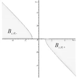
Now we need the spectrum of the operator Dc,γ(θ). Theorem 1 shows (see Figure 1)σ(Dc,0(θ)) = Σ−c(θ)∪Σ+c(θ), where Σ±c(θ) =±Ec(R;θ).
In the case of self-adjoint operators the compactness of the difference of free and interacting resolvent would imply that Dc,0(θ) and Dc,γ(θ) with γ 6= 0
have the same essential spectrum. This is however not true for non-self-adjoint operators in general. In particular there exist several different definitions of the essential spectrum, which do not coincide in general and have different invariance properties.
In the case of relatively compact perturbations this difficulty can be mastered using the analytic Fredholm theorem [50]. Since Coulomb type potentials are not relatively compact, we adapt a strategy invented by Nenciu [40] for the self-adjoint case. We need the following lemma:
Lemma2. Let θ∈Sπ/4andz /∈σ(Dc,0(θ)). Then the operatorVC1/2(Dc,0(θ)−
z)−1 is compact.
Proof. It suffices to consider the case z = 0. We write VC1/2Dc,0(θ)−1 =
VC1/2 √
−c2e−2θ∆ +c4β−1√−c2e−2θ∆ +c4βDc,
0(θ)−1. Because of
VC1/2∈L6
w(R3) and 1/(± p
c2e−2θ(·)2+c4−z)∈L6(R3), the operator
VC1/2(√−c2e−2θ∆ +c4β−z)−1is compact [44]. Moreover, Theorem 1 implies
(√−c2e−2θ∆ +c4β)Dc,
0(θ)−1k ≤1 +CFW|Imθ|.This shows the claim.
Forz /∈σ(Dc,0(θ)) we define the operatorMc;θ(z) :=V2(θ)(Dc,0(θ)−z)−1V1(θ).
Moreover, let Bc;θ;+ and Bc;θ;− (see Figure 1) the closed subsets of {z ∈
Figure 1: The spectrum of the operatorDc,0(θ) and setsBc;θ;± forc= 1 and θ= iπ/4.
curves [c2,∞) and Ec(R;θ) ((−∞,−c2] and −Ec(R;θ) respectively). We set
Bc;θ=Bc;θ;+∪Bc;θ;−.
Furthermore, forθ∈Sπ/4 we define the constants
C(Imθ) := 1 +pCFW|Imθ|
cos(2Imθ) , C1(Imθ) :=C(Imθ) +
1 +CFW|Imθ|
cos(Imθ) . (24) Note the inequality 1/cos(Imθ)≤C(Imθ).
The following theorem yields a precise description of the spectrum of the op-erator Dc,γ(θ). In particular, outside the set Bc,θ the spectra ofDc,γ(θ) and Dc,γ(0) coincide so that one particle resonances – if any exist – can be located only within the setBc,θ.
LetB(L2(R3;C4)) be the set of bounded and everywhere defined operators on
L2(R3;C4). Moreover, we setBa(x
0) :={x∈R3||x−x0|< a} fora >0 and
x0∈R3
Theorem 3. Let θ ∈ Smin{π/4,Θ} and 2cγC(Imθ) < 1. Suppose that (H1)
holds. Then σ(Dc,γ(θ)) =σ(Dc,0(θ))∪Ac,γ;θ,whereAc,γ;θ is a discrete subset
ofC\σ(Dc,0(θ), and we haveAc,γ;θ∩(C\Bc;θ) =σdisc(Dc,γ(0)). The setAc,γ;θ
has at most the accumulation points ±c2. For z /∈ σ(Dc,γ(θ)) the resolvent
identity
(Dc,γ(θ)−z)−1= (Dc,0(θ)−z)−1+
+γ(Dc,0(θ)−z)−1V1(θ)(1−e−θγMc;θ(z))−1V2(θ)(Dc,0(θ)−z)−1 (25)
holds.
Step 1: Proof of (25)forz= iη,η∈R. Using Kato’s inequality and Theorem 1 we obtain
kγMc;θ(iη)k=kγV2(θ)(Dc,0(θ)−iη)−1V1(θ)k ≤
γπe−Reθ(1 +C
FW|Imθ|)
2
× kp |∇|
−cos(2Imθ)c2e−2Reθ∆ +c4k ≤
γ c
π
2C(Imθ), (26) where we used additionally (5) and Lemma 1. Equation (26) shows that (25) holds forz= iη,η ∈R.
Step 2: Proof of (25), general case. We have
1−γMc;θ(z) = 1−γMc;θ(0)−γ(Mc;θ(z)−Mc;θ(0)) = (1−γMc;θ(0))(1−N(z)),
where N(z) := z(1−γMc;θ(0))−1V2(θ)Dc,0(θ)−1(Dc,0(θ)−z)−1V1(θ).
Us-ing Step 1 and Lemma 2 we see that N(z) is compact and a holomorphic function of z for z ∈ C\σ(Dc,0(θ)). Applying the analytic Fredholm
the-orem [41, Thethe-orem VI.14] yields that (1−N(z))−1 is a meromorphic
func-tion on C\σ(Dc,0(θ)) with values in B(L2(R3;C4)), whose residues are
op-erators of finite rank. Using Step 1 once more, we see that this also holds for (1−e−θγMc;θ(z))−1. In particular, there is a setAc,γ;θ ⊂C\σ(Dc,0(θ))
which has no accumulation point in C\σ(Dc,0(θ)) such thatz 7→Rc,γ;θ(z) is
holomorphic inC\(σ(Dc,0(θ))∪Ac,γ;θ).
Step 3: The mapping z 7→ Rc,γ;θ(z) (Dc,γ(θ)−z)f with f ∈ Dom(Dc,γ(θ))
is holomorphic on C\(σ(Dc,0(θ))∪Ac,γ;θ). Because of Step 1 the operator
Rc,γ;θ(z) equals the resolvent of Dc,γ(θ) for z = iη, η ∈ R. It follows that
Rc,γ;θ(z) (Dc,γ(θ)−z)f = f for all z ∈ C\(σ(Dc,0(θ))∪Ac,γ;θ) and f ∈
Dom(Dc,γ(θ)).
Moreover, it is easy to see that RanRc,γ;θ(z)⊂H1/2(R3;C4). Thus, we obtain
as before (g,(Dc,γ(θ)−z)Rc,γ;θ(z)f) = (g, f) for all f ∈ L2(R3;C4), g ∈
H1/2(R3;C4) andz∈C\(σ(Dc,
0(θ))∪Ac,γ;θ). It follows that RanRc,γ;θ(z)⊂
H1(R3;C4) and (Dc,γ(θ)−z)Rc,γ
;θ(z)f = f forf ∈ L2(R3;C4) andz ∈C\
(σ(Dc,0(θ))∪Ac,γ;θ). Summarizing, we find Rc,γ;θ(z) = (Dc,γ(θ)−z)−1 for
all z ∈ C\(σ(Dc,0(θ))∪Ac,γ;θ). In particular, it follows that σ(Dc,γ(θ)) ⊂
σ(Dc,0(θ))∪Ac,γ;θ.
Let nowz0∈Ac,γ;θ. Then the analytic Fredholm theorem implies the existence
off ∈L2(R3;C4) with (1−N(z
0))f = 0, and thus also (1−γMc;θ(z0))f = 0.
We proceed as follows: Since (Dc,0(θ)−z)−1V1(θ) is bounded, we find f ∈
Ran(V2(θ)), i.e. f = V2(θ)g for g = (Dc,0(θ)−z)−1V1(θ)f ∈ L2(R3;C4). It
follows that (Dc,0(θ)−z0)g =γV1(θ)f =γV(θ)g in H−1/2(R3;C4).
Rewrit-ing this equality (in the sense of H−1/2(R3;C4)) we find −ice−θα· ∇g − βc2g−γV(θ)g = z0g. Since the r.h.s. of this equality is a (regular
distri-bution generated by a) function inL2(R3;C4), the l.h.s. is. This implies that
g∈H1(R3;C4) =
D(Dc,γ(θ)) by Remark 2, i.e. z0∈σ(Dc,γ(θ)) which in turn
Step 4: It remains to show that σ(Dc,γ(θ))∩σ(Dc,0(θ)) = σ(Dc,0(θ)) holds.
To show this, we pick E ∈σ(Dc,0(θ)) and p∈R3 with E =Ec(p;θ) in order
to construct a suitable Weyl sequence. Let us defineψp,c;θ∈C∞(R3;C4) by ψp,c;θ(x) :=Nc(p;θ)−1(c2+Ec(p;θ)ξ, ce−θσ·pξ)Te−ipx (27) withξ= (1,0)T.Equations (7) and (23) imply
(−icα· ∇+βc2)ψp,c;θ(x) =Ec(p;θ)ψp,c;θ(x). (28) We pick a function 06=φ ∈C0∞(R3) with suppφ ⊂B1(0) and set forn∈ N
φn(x) :=φ(n1x−ne1) withe1= (1,0,0)T as well asfn:=φnψp,c;θ.Obviously,
we havefn∈Dom(Dc,γ(θ)). First, we calculate
kfnk ≥(1 +CFW)−1/2kφnk=n3/2(1 +CFW)−1/2kφk, (29)
where we used the definition (27) ofψp,c;θ, Equation (7), Equation (11),
Equa-tion (8) and the identity R
dx φn(x)2 = R dx φ(1
nx−ne1) = n
3R
dx φ(x)2.
Furthermore, we find forn≥2
kVCfnk2= Z
dx 1
|x|2φn(x) 2
kψp,c;θ(0)k2 (30) ≤(1 +CFW|Imθ|)
4 n4
Z
dx φn(x)24(1 +CFW|Imθ|)
n4 n
3kφk2,
since suppφn ⊂Bn(n2e
1) andkψp,c;θ(0)k ≤p1 +CFW|Imθ| because of
For-mula (9). Moreover, we obtain
k(cα· ∇φn)ψp,c;θ(·)k ≤ c p
1 +CFW|Imθ|
n n
3/2
k∇φk. (31) Formulas (28) through (31) imply
k(Dc,γ(θ)−Ec(p;θ))fnk kfnk ≤
p
1+CFW|Imθ| 2n3/2
n2 kφk+cn 3/2
n k∇φk n3/2
√
1+CFWkφk
−→
n→∞ 0. Thus Dc,γ(θ)−Ec(p;θ) does not have a bounded inverse and Ec(p;θ) ∈
σ(Dc,γ(θ)).
Step 5: The proof ofAc,γ;θ∩(C\Bc;θ) =σdisc(Dc,γ(0)) is a standard argument,
which uses the dilation analyticity of the operators Dc,γ(θ) (see [43, Chapter XII.6] or [46]). The same holds for the claim on the accumulation points.
Remark3. Note that forV =VC the set of resonances is empty. This follows similarly as for the Schr¨odinger case (see [8]): If there was a resonance, then
5 Spectral Projections
In this section we extend the notion of positive and negative spectral projections to dilated Dirac operators. We define for p∈ R3 the matrices Λ(±)
following definition for the dilated interacting operators:
Λ(c,γ±)(θ) := It is well known [33, Chapter VI-5.2, Lemma 5.6] that Equation (32) yields the positive and negative spectral projections for realθ. Note that similar formulas for not necessarily self-adjoint operators are known (see [16, Chapter VX]). These authors use a different definition for the spectral projections, however. First, we show in Theorem 4 that these operators are well defined and bounded projections even ifθ /∈R. We need the following technical lemma:
Lemma 3. Letθ∈Sπ/4. Then for all η∈R k|Dc,Dc,0(Reθ)| −iη
0(θ)−iη k ≤C1(Imθ), (33)
whereC1(Imθ) is defined in (24).
Proof. We prove the estimate
k√ |Dc,0(Reθ)| −iη
Proof. The proof is inspired by similar estimates in [47].
Step 1: The resolvent equation (25) and the estimate (26) yield the convergence of the series
Step 2: We show that the expression
lim
Step 4: We show that the limit exists as a strong limit and estimate for g ∈
Here we estimated the expression in the square brackets similarly to (26), but used Hardy’s inequality instead of Kato’s inequality. Moreover, we used the estimate (33) twice. Sinceσ(Dc,0(Reθ)) = (−∞, c2]∪[c2,∞), we have
This estimate shows that the convergence in formula (36) is uniform in f ∈
L2(R3;C4), which implies the strong convergence [33, Theorem III.1.32 and
Lemma III.3.5], sinceH1/2(R3;C4) is dense inL2(R3;C4).
Obviously, the identity Λ(+)c,γ(θ) + Λ(c,γ−)(θ) = 1 holds. We set Hc,γ(±)(θ) := Λ(c,γ±)(θ)L2(R3;C4) and findL2(R3;C4) =Hc,γ(+)(θ)∔Hc,γ(−)(θ), wehre∔denotes the direct sum. We call the Λ(c,γ±)(θ) positive and negative spectral projections and H(c,γ±)(θ) positive and negative spectral subspaces, respectively. This is justified because of Theorem 5.
The following corollary generalizes [47, Lemma 1] to dilated spectral projec-tions.
Proof. This follows directly from Equation (37) in the proof of Theorem 4. The next theorem shows that the spaces Hc,γ(±)(θ) are invariant underDc,γ(θ) and describes the spectrum of the restriction of the operator to these spaces. If a part of the spectrum is contained in a Jordan curve, analogous statements can be found in [33, Theorem III-6.17]. The following theorem describes a more general situation, but the essential elements of the proof of [33, Theorem III-6.17] can be adapted.
Theorem5. Letθ∈Smin{π/4,Θ}and 2cγC(Imθ)<1. Suppose that (H1) holds.
Then the identity
Λ(±)
c,γ(θ)(Dc,γ(θ)−z)−1= (Dc,γ(θ)−z)−1Λ(c,γ±)(θ) (38)
holds for all z ∈ρ(Dc,γ(θ)). The subspaces Ran Λ(+)c,γ(θ) andRan Λ(c,γ−)(θ) are
invariant subspaces for Dc,γ(θ). In particular,
σ(Dc,γ(θ)|Ran Λ(+)
c,γ(θ)) =σ(Dc,γ(θ))∩ {z∈C|Rez >0} (39)
and
σ(Dc,γ(θ)|Ran Λ(−)
c,γ(θ)) =σ(Dc,γ(θ))∩ {z∈C|Rez <0} (40)
hold.
Proof. Obviously, for allz /∈σ(Dc,γ(θ)), all η∈Rand all f ∈L2(R3;C4) the
equation (Dc,γ(θ)−z)−1(Dc,γ(θ)−iη)−1f = (Dc,γ(θ)−iη)−1(Dc,γ(θ)−z)−1f
is true. This immediately implies
(Dc,γ(θ)−z)−1 lim R→∞
Z R −R
dη (Dc,γ(θ)−iη)−1f =
= lim R→∞
Z R −R
dη (Dc,γ(θ)−iη)−1(Dc,γ(θ)−z)−1f
and thus (38). It follows that [33, Chapter III-5.6 and Theorem III.6.5] (Dc,γ(θ) − z)−1Ran Λ(±)
c,γ(θ) ⊂ Ran Λ(c,γ±)(θ) and Λ(c,γ±)(θ) Dom(Dc,γ(θ)) ⊂ Dom(Dc,γ(θ)) as well as Dc,γ(θ)H(c,γ±)(θ) ⊂ H(c,γ±)(θ). We define the operators D(c,γ±)(θ) :=Dc,γ(θ)|H(±)
c,γ(θ) and (for z /∈σ(Dc,γ(θ)) at the moment) the
resol-vents R(c,γ±);θ(z) := (D(c,γ±)(θ)−z)−1 = (Dc,γ(θ)−z)−1|H(±)
c,γ(θ). In particular,
σ(Dc,γ(±)(θ))⊂σ(Dc,γ(θ)).
On the other side, we have f ∈ H(c,γ±)(θ) and z /∈ σ(Dc,γ(θ)) R(c,γ±);θ(z)f = (Dc,γ(θ)−z)−1f = (Dc,γ(θ)−z)−1Λ(±)
c,γ(θ)f. Using the first resolvent identity, we find forz∈Cwith Rez <0 respectively Rez >0
(Dc,γ(θ)−z)−1Λ(c,γ±)(θ)f =− 1 2π
Z ∞
−∞ dη 1
z−iη(Dc,γ(θ)−iη)
−1f, (41)
since forz∈Cwith Rez <0 respectively Rez >0 the residue theorem implies limR→∞R−RRdη
1
z−iη = limR→∞ RR
−Rdη z
z2+η2 =∓π.
0} ⊂ ρ(D(c,γ−)(θ)). This proves σ(Dc,γ(−)(θ)) ⊂ {z ∈ C|Rez < 0} and σ(Dc,γ(+)(θ)) ⊂ {z ∈ C|Rez > 0}. On the other side, z ∈ σ(Dc,γ(θ)) cannot fulfill both z∈ρ(D(c,γ−)(θ)) andz∈ρ(Dc,γ(+)(θ)), because otherwise the identity (Dc,γ(θ)−z)−1= (D(+)
c,γ(θ)−z)−1Λ(+)c,γ(θ)+(Dc,γ(−)(θ)−z)−1Λ(c,γ−)(θ) would imply the contradictionz∈ρ(Dc,γ(θ)). This shows (39) and (40).
Next, we need spectral projections for the eigenvalues: We define for alln≥1 (andn≤Nmax if there only finitely many eigenvalues) the spectral projections
Pn(c, γ;θ) :=− 1
2πi Z
Γn(c,γ)
1
Dc,γ(θ)−zdz , (42) wherezruns through Γn(c, γ) in the positive sense. Γn(c, γ) is chosen such that for all 1 ≤l ≤ Nn the eigenvalues ˜En,l(c, γ) are located within the contour, but no other elements of the spectrumDc,γ(θ).
For later, we need spectral projections for the fine structure components. We set forn≥1 and 1≤l≤Nn
Pn,l(c, γ;θ) :=− 1
2πi Z
Γn,l(c,γ)
1
Dc,γ(θ)−zdz , (43) where z runs through Γn,l(c, γ) in the positive sense, and Γn,l(c, γ) is chosen such that only the eigenvalue ˜En,l(c, γ) lies within the contour. We denote the corresponding normed eigenfunctions byφn,l(c, γ;θ).
6 Transformation Functions
We need transformation functions between the spectral subspaces of dilated and not dilated operators for the resolvent estimate in Section 7 and in order to establish the dilation analyticity of a relativistic Pauli-Fierz model in [30]. Another example for a transformation function is the Douglas-Kroll transfor-mation, which was investigated by Siedentop and Stockmeyer [47] (see also Huber and Stockmeyer [31]). Contrary to the situation there, our spectral projections are not self-adjoint and thus the transformation function is a non-unitary similarity transformation. The estimates in this section can be used to generalize the Douglas-Kroll transformation to complex dilated operators. In order to prove the existence of the transformation function, we need norm estimates on the difference between the spectral projections.
Lemma 4. Let θ ∈Smin{π/4,Θ}. Suppose that (H1) and (H2) hold. Then the
following statements hold:
a) There is a constant CDL >0 (independent of c, γ and θ) such that for 2γ
c C(Imθ)<1 the estimate
kΛ(±)
holds. The operator|Dc,0(0)|1/2[Λ(c,γ±)(0)−Λ(c,γ±)(θ)]|Dc,0(0)|−1/2is a
holo-morphic function ofθ∈Mγ/c.
b) Let moreover0< q <1. Then there is a constantCDLS>0(independent
ofc,γ andθ) such that for 2cγC(Imθ)< q the estimate
k|Dc,0(0)|1/2[Λc,γ(±)(0)−Λc,γ(±)(θ)]|Dc,0(0)|−1/2k ≤CDLS|θ| (45)
holds.
Proof. We adapt method which was used by Siedentop and Stockmeyer [47]
and by Griesemer, Lewis and Siedentop [19] for other choices of projections. We start with the difference of resolvents
(Dc,0(θ)−iη)−1−(Dc,0(0)−iη)−1
=ic[e−θ−1](Dc,0(θ)−iη)−1α· ∇(Dc,0(0)−iη)−1 (46) and note that|e−θ−1| ≤B|θ| holds withB=eπ/4 for all|θ| ≤π/4.
Step 1: Proof for the free projections. Equation (46) it and Lemma 3 imply that
|(f,[(Dc,0(θ)−iη)−1−(Dc,0(0)−iη)−1]g)|
≤B|θ|k|Dc,0(Reθ)|1/2(|Dc,0(Reθ)|+ iη)−1fkk|Dc,0(0)|1/2(Dc,0(0)−iη)−1gk × k|Dc,0(Reθ)|−1/2cα· ∇|Dc,0(0)|−1/2kk|Dc,0(Reθ)| −iη
Dc,0(θ)−iη k ≤ B|θ|
e−Reθ/2C1(Imθ)k
|Dc,0(Reθ)|1/2 |Dc,0(Reθ)|+ iη
fkk|Dc,0(0)| 1/2
Dc,0(0)−iη
gk,
where we used the estimatekc|∇||Dc,0(Reθ)|−1k ≤1/e−Reθ.
This proves (cf. [47, Proof of Lemma 1] and proof of Corollary 1) kΛ(c,±0)(0)−
Λc,(±0)(θ)k ≤ C˜DL|θ| with a ˜CDL > 0 and analogously k|Dc,0(0)|1/2[Λ(c,±0)(0)−
Λc,(±0)(θ)]|Dc,0(0)|−1/2k ≤C˜DL|θ|,since|Dc,0(0)|1/2commutes with all operators
in (46).
Step 2: Proof of (44). We write
V2(θ) 1
Dc,0(θ)−iη
V1(θ)−V2(0) 1
Dc,0(0)−iη
V1(0) (47)
≤
V1(θ)
e−θ Dc,0(θ)−iη
χθV2(θ)−V1(θ)
e−θ Dc,0(0)−iη
χθV2(θ)
+
VC1/2 1 Dc,0(0)−iη
(χθe−θ−1)VC1/2 ≤
B|θ|π
where we estimated the second summand by B(1 + ˜C)|θ|π/(2c) from above, and the second summand – similarly as in (26) – according to
In the same way we obtain
Formulas (47) through (50) show
Step 3: Proof of (45). We use the expansion
and start with the necessary estimates on the differences of the resolvents: Using Hardy’s inequality, we obtain as in (26)
k[V(θ)(Dc,0(θ)−iη)−1−V(0)(Dc,0(0)−iη)−1]|Dc,0(0)|−1/2g For the terms with the resolvents we use Lemma 3 and Lemma 1 to estimate
Formulas (52) through (56) show
γn which in turn proves (45).
Step 4: Holomorphicity. This follows as in the proof of Theorem 4, since f,|Dc,0(0)|1/2Dc,0(1θ)−iηV(θ)Dc,0(1θ)−iη
n−1
V(θ)Dc,0(1θ)−iη|Dc,0(0)|−1/2gare
Before we turn to the existence of a transformation function in Theorem 6, we need two operator inequalities, one of which was proven in [19]. Since the other inequality can be proven completely analogously, we omit the proof. Let us mention that there exits an improved version of one of these inequalities (see [39]). But since we will be interested in the non-relativistic limit only, it is sufficient to use the original version.
Lemma5 ([19], Lemma 2). Suppose thatϑ∈Rand γc < 12. Then the operator inequalities
(1−2γc )|Dc,0(ϑ)k ≤ |Dc,γ(ϑ)| ≤(1 +
2γ
c )|Dc,0(ϑ)|
hold.
Now we can turn to the transformation functionUDL(c, γ;θ) defined below. It
enables us to consider the operatorUDL(c, γ;θ)Dc,γ(±)(θ)UDL(c, γ;θ)−1instead of
the operatorD(c,γ±)(θ). This is necessary for technical reasons, since the latter operates on a fixed space (i.e. Ran Λ(+)c,γ(0)). We will prove in [30] that this operator defines a holomorphic family of operators. Moreover, we will need the transformation function in the proof of the resolvent estimate in Theorem 7.
Theorem 6. Suppose that θ ∈ Smin{π/4,Θ}, 2cγC(Imθ) <1 and CDL|θ| < q
for some 0 < q < 1. Suppose moreover that (H1) and (H2) hold. Then the following statements hold:
a) There is a bounded mapping UDL(c, γ;θ) :L2(R3;C4)→L2(R3;C4)with
the property
UDL(c, γ;θ)Λ(+)c,γ(θ)UDL(c, γ;θ)−1= Λ(+)c,γ(0) (57)
and bounded inverse VDL(c, γ;θ) := UDL(c, γ;θ)−1. There is a constant
CUDL >0, independent ofc,γ andθ, such that
kUDL(c, γ;θ)−1k ≤CUDL|θ| (58)
holds.
b) Suppose that additionally CDLS|θ| < q holds. Then there is a constant
CUDLS, independent of c,γ andθ, such that
k|Dc,0(0)|1/2UDL(c, γ;θ)|Dc,0(0)|−1/2−1k ≤CUDLS|θ| (59)
is true. The same estimates hold forVDL(c, γ;θ).
c) The operator UDL(c, γ;θ), and for CDLS|θ|< qthe operator |Dc,0(0)|1/2UDL(c, γ;θ)|Dc,0(0)|−1/2
and the operator |Dc,0(0)|−1/2UDL(c, γ;θ)|Dc,0(0)|1/2, are holomorphic
Proof. We follow [47, Theorem 1] and [33, Chapter I-4.6.] and define
has a norm convergent series expansion for bounded operatorsAwithkAk<1.
Proof of (58): We follow [47, Proof of Lemma 5]. We have Λ(+)c,γ(0)Λ(+)c,γ(θ) +
Lemma 4 implies that the estimatesk
Λ(c,γ−)(0)−Λ(+)c,γ(0)Λ(+)c,γ(θ)−Λ(+)c,γ(0)k ≤
Proof of (59): The strategy is similar to the proof of (58). We write
where we used that|Dc,γ(0)|−1/2commutes with Λ(±)
c,γ(0). Using Lemma 5 and Lemma 4 we obtain the claim as before.
A first application of the transformation functionUDL(c, γ;θ) is the following
lemma, which estimates the difference between the dilated Dirac operator and its original version.
Lemma6.Under the assumptions of Theorem 6 b) there is a constantCUD >0, independent of γ,c andθ, such that
|Dc,0(0)| −1/2
UDL(c, γ;θ)Dc,γ(θ)UDL(c, γ;θ)−1 −Dc,γ(0)
|Dc,0(0)|−1/2
≤CUD|θ| (61)
holds.
Proof. We have
|Dc,0(0)|−1/2[UDL(c, γ;θ)Dc,γ(θ)UDL(c, γ;θ)−1−Dc,γ(0)]|Dc,0(0)|−1/2
=|Dc,0(0)|−1/2[UDL(c, γ;θ)−1]|Dc,0(0)|1/2|Dc,0(0)|−1/2Dc,γ(θ)|Dc,0(0)|−1/2 ×|Dc,0(0)|1/2UDL(c, γ;θ)−1|Dc,0(0)|−1/2+
+|Dc,0(0)|−1/2[Dc,γ(θ)−Dc,γ(0)]|Dc,0(0)|−1/2
×|Dc,0(0)|1/2UDL(c, γ;θ)−1|Dc,0(0)|−1/2+|Dc,0(0)|−1/2Dc,γ(0)|Dc,0(0)|−1/2 ×|Dc,0(0)|1/2[UDL(c, γ;θ)−1−1]|Dc,0(0)|−1/2,
which implies the claim, if we use additionally
k|Dc,0(0)|−1/2[Dc,γ(θ)−Dc,γ(0)]|Dc,0(0)|−1/2k=k|Dc,0(0)|−1/2 (62) ×[−(e−θ−1)icα· ∇ −γ(V(θ)−V)]|Dc,0(0)|−1/2k ≤(B+ ˜C)|θ|(1 + πγ
2c) and Theorem 6. Moreover, we used the inequality |e−θ−1| ≤B|θ|with B = eπ/4and Kato’s inequality in the proof of (62).
7 A resolvent estimate for the Dirac operator
In the following, we choose anη >0 such that for some ˜n >1 and allc≥1 the inequalities ˜En,˜n(c, γ)˜ < c2−η and ˜En˜+1,1(c, γ)> c2−η hold. If ˜n=Nmax,
then the second condition has to be omitted.
Using the notation of Section 5 we definePdisc,n˜(c, γ;θ) :=P1≤n≤˜nPn(c, γ;θ)
and ¯Pdisc,n(c, γ;˜ θ) :=1−(Λ(c,γ−)(θ) +Pdisc,n˜(c, γ;θ)). Note that ¯Pdisc,n(c, γ;˜ θ)
The following theorem partly generalizes [5, Lemma 3.8] for Dirac operators (see also Theorem A.1). We will slightly extend this theorem in the non-relativistic limit (see Lemma 7 and Corollary 4). This theorem and Corollary 4 enable us to control the norm of the resolvent of the non-self-adjoint operator Dc,γ(θ)|Ran ¯Pdisc,n˜(c,γ;θ). Note that the usual theorems about the norm of the
resolvent of a self-adjoint operator fail in general, and that for the following to hold it is essential that to restrict the operator to (a subspace of) the positive spectral subspace.
Theorem 7. Suppose that the assumptions of Theorem 6 b) hold. Assume additionally that the inequalitiesCUD|θ|(1+2γ/c)< qand2γ(1+CFW|Imθ|)<
qare fulfilled for some0< q <1. Then the following statements are true: The operator Dc,γ(θ)|Ran ¯Pdisc,˜n(c,γ;θ)−z has a bounded inverse for all z ∈C with
Proof. We make a case distinction:
Case 1: Rez≤0. Theorem 6 implies the inclusion Ran(UDL(c, γ;θ)
As in [5, Proof of Lemma 3.8], we use a resolvent expansion: [(UDL(c, γ;θ)Dc,γ(θ)UDL(c, γ;θ)−1)|Ran Λ(+)
In order to prove the convergence of the series, we have to estimate the terms in (63). First, we note that
holds, since Rez≤0. Moreover, the spectral theorem implies
Lemma 6, Lemma 5 and (64) prove the convergence of the series in (63). Using Formula (65), the claim follows for Rez≤0 from (63).
Case 2: 0≤Rez≤c2−1. We use the resolvent expansion
2−1). If we differentiate this function, we find that it
attains its maximum at the pointr0:=
√ c4−l2c
l . Now, we define the function gc(l) := fc,l(r0) = √c4c−l2 for 0 ≤ l ≤ (c
2−1). This function is obviously
monotonously increasing inl and therefore attains its maximum at the point l0:=c2−1. We havegc(l0) = √ c
8.1 General Theory
We extend some statements from [49] to the non-self-adjoint case. We define β±:= 12(1±β) as well asM :={z∈C| −1≤Rez <0,|Imz| ≤1}and fix a γ >0 such thatDc,γ(θ)−c2 has no eigenvaluesEwith ReE≤ −1. This is at
least true for 0≤γ <1 in the case ofV =VC, which can be seen, for example, using the explicit formula for the eigenvalues, see [35]. We define as operators onL2(R3;C4):
D∞,0(θ) :=−
e−2θ
2 ∆, D∞,γ(θ) :=− e−2θ
2 ∆−γV(θ)β+ Kc,0(θ) := (D∞,0(θ)−z− z
2
2c2)−
1, Kc,γ(θ) := (D
∞,γ(θ)−z− z
2
2c2)− 1
as well as
R∞,0;θ(z) := (D∞,0(θ)−z)−1, Rc,0;θ(z) := (Dc,0(θ)−z)−1
R∞,γ;θ(z) := (D∞,γ(θ)−z)−1, Rc,γ;θ(z) := (Dc,γ(θ)−z)−1.
First, we generalize [49, Theorem 6.1 and Theorem 6.4] to dilated operators. As in [49], Theorem 8 is the starting point for the investigation of the non-relativistic limit.
Theorem 8. a) Suppose thatθ∈Sπ/4andc≥1. Then forz /∈σ(Dc,0(θ))∪
σ(D∞,0(θ))the resolvent relation
(Dc,0(θ)∓c2−z)−1=
β±±2c12(−icα· ∇ ±z)
×
1∓2c12z 2(
±D∞,0(θ)−z)−1
−1
(±D∞,0(θ)−z)−1 (67)
holds.
b) Suppose that θ∈Smin{π/4,θ}, 2cγC(Imθ)<1 and that (H1) holds. Then
forz∈M \Rthe relations
(Dc,γ(θ)−c2−z)−1=
β++
1
2c2(−ice−
θ
α· ∇+z)
×Kc,γ(θ)1−2cγ2V(θ)(−ice−
θα
· ∇+z)Kc,γ(θ)−
1
(68)
and
Kc,γ(θ) =
1− z 2
2c2(D∞,γ(θ)−z)− 1
−1
(D∞,γ(θ)−z)−1 (69)
Proof.
a) We follow the proof of [49, Theorem 6.1], noting thatz∈Cwithz(1+ z
2c2)∈/
e−2i Imθ[0,∞) is equivalent toz+c2 ∈/ σ(Dc,
0(θ)). In order to show Equation
(67), we define the operatorsA±(θ) :=Dc,0(θ)±c2±z=−icα· ∇ ±2c2β±±z
which in turn implies the claim. Note that all operators are equivalent to multiplication operators.
b) We follow the proof of [49, Theorem 6.2]. Theorem 3 implies that z+c2 ∈/ σ(Dc,γ(θ)). It follows that Dc,γ(θ)−(c2+z) = A
−(θ)−γV(θ) = (1+γV(θ)A−(θ)−1)A
−(θ).SinceDc,γ(θ)−(c2+z) andA−(θ) have bounded inverses, the bounded operator 1+γV(θ)A−(θ)−1 is bijective, and is thus in
particular bounded invertible. From Equation (70) it follows that
(Dc,γ(θ)−c2−z)−1= (A−(θ)−γV(θ))−1=A−(θ)−1(1−γV(θ)A−(θ)−1)−1
σ(D∞,0(θ)), i.e. Kc,0(θ) is bounded invertible. Thus, the bounded operator
1−γV(θ)β+Kc,0(θ)−1 has a bounded inverse, and hold. Using (72) and (73), (68) follows from (71).
eigenvalues are the same as the eigenvalues of D∞,γ(0) and that |En(∞, γ)−
En,l(c, γ)|=O(1/c2) for alll∈ {1, . . . , Nn}by [49, Theorem 6.8]. We pick now
η as in Section 7 and define for each ˜ǫ >0 the set
Mη,˜ǫ:={z∈C|1≤Rez≤ −(η+ ˜ǫ), |Imz| ≤1, dist(z, σ(Dc,γ(θ)))≥˜ǫ}. Moreover, we set D(w, r) := {z ∈ C||z−w| < r} for w ∈C and r > 0. Fix ˜
ǫ > 0 so small that for all n, n′ ∈ N with n 6= n′ and 1 ≤ n, n′ ≤ ˜n the sets D(En(∞, γ),2˜ǫ) and D(En′(∞, γ),2˜ǫ) are disjoint and contained in the
set {z∈C|1≤Rez≤ −(η+ ˜ǫ), |Imz| ≤1}. Now we pick for ˜ǫ >0 a contour Γ with positive orientation such that Γ is contained Mη,˜ǫ and has only the eigenvalueEn(γ) in its interior, but no other eigenvalues ofσ(D∞,γ(θ)). Then we define
Pn(∞, γ;θ) :=−2πi1
Z
Γ
dz R∞,γ;θ(z)β+.
We set Pdisc(∞, γ;θ) := P˜ni=1Pi(∞, γ;θ) and ¯Pdisc(∞, γ;θ) := 1 −
Pdisc(∞, γ;θ). Note that using the definitions in Appendix A and in slight
abuse of notation Pdisc(∞, γ;θ) = Pdisc(γ;θ)β+ and ¯Pdisc(∞, γ;θ) = β− + ¯
Pdisc(γ;θ)β+.
Now we are in the position to generalize [49, Corollary 6.5] to dilated operators.
Corollary 2. Suppose that |θ| < θ0, whereθ0 is sufficiently small (see
Ap-pendix A), and θ ∈Smin{π/4,Θ} as well as 2cγC(Imθ)<1. Suppose moreover
that (H1) holds. Then the resolvent expansion
Dc,γ(θ)−(c2+z)−1= ∞ X
n=0
1
cnRn(z). (74)
holds for allz∈Mη,ǫ˜and all sufficiently largec. The series converges in norm,
uniformly in θ andz. In particular,
[Dc,γ(θ)−(c2+z)]−1 −→
c→∞[D∞,γ(θ)−z] −1β
+
uniformly in θ andz.
Proof. First, we need an estimate on the resolvent ofD∞,γ(θ). We split the resolvent according to
[D∞,γ(θ)−z]−1= [D∞,γ(θ)|Ran ¯Pdisc(∞,γ;θ)−z]
−1P¯
disc(∞, γ;θ) (75)
+
˜
n X
n=1
[D∞,γ(θ)|RanPn(∞,γ;θ)−z]
−1Pn(
∞, γ;θ).
Theorem A.1 implies that the norm of the first summand in (75) is bounded by 2/η. The norms of the other summands can be estimated according to
[D∞,γ(θ)|RanPn(∞,γ;θ)−z]−
1Pn(∞, γ;θ) ≤ k
Pn(∞,γ;θ)k dist(z,En(γ)) ≤
C|θ|
Corollary A.1. Thus, we have for sufficiently small 1/c (dependent on ˜ǫ) and allz∈Mη,ǫ˜the expansion
(1− z 2
2c2(D∞,γ(θ)−z)−
1)−1= (D
∞,γ(θ)−z)−1 ∞ X
n=0
(z
2
2c2(D∞,γ(θ)−z)− 1)n.
Hardy’s inequality implies forf ∈H2(R3;C4) the estimateskV fk ≤2k∇fk ≤
ak∆fk+ (1/a)kfk and e−2Reθk∆fk ≤ 1/(1−2aγ)kD
∞,γ(θ)fk+ 2γ/[a(1− 2aγ)]kfkwith a sufficiently smalla >0. It follows that
k γ
2c2V(θ)(−ice
−θ
α·∇+z)(D∞,γ(θ)−z)−1k ≤ γ
c[C1+C2k(D∞,γ(θ)−z) −1
k]
holds with C1, C2 > 0 (independent of γ, c and θ), which implies that the
last factor in (68) has a norm convergent series expansion in 1/cfor 1/csmall enough.
Remark4. We findR0(z) :=β+R∞,γ;θ(z)as in [49]. As in [49, Remark after
Corollary 6.5], the operators occurring with even powers of 1/care even, and the operators occurring with odd powers of1/care odd .
Lemma 7. Suppose that the assumptions of Corollary 2 hold. Then there is a constant CP,n >0 (independent of c and θ) such that for sufficiently large c
the estimate
kPn(c, γ;θ)−Pn(∞, γ;θ)k ≤ CPc,n
holds.
Proof. This follows immediately from Corollary 2. The following two corollaries extend Theorem 7.
Corollary 3. Suppose that the assumptions of Corollary 2 hold. Then there is a constant C > 0 (possibly dependent on θ) such that for all z ∈ C with
−1≤Rez≤ −η and|Imz| ≤1 and all sufficiently largec the estimate
k[Dc,γ(θ)|Ran ¯Pdisc,n˜(c,γ;θ)−(c
2+z)]−1P¯
disc,n(c, γ;˜ θ)k ≤C
holds.
Proof. Corollary 2 implies that [Dc,γ(θ)|Ran ¯Pdisc,˜n(c,γ;θ)−(c
2+z)]−1is uniformly
bounded in z ∈Mη,ǫ˜andc (for sufficiently largec). Lemma 7 and Lemma 4
yield the existence of an upper bound on
kP¯disc,˜n(c, γ;θ)k=k1−(Λ(c,γ−)(θ) +Pdisc,n(c, γ;˜ θ))k,
Letz0∈D(En(∞, γ),˜ǫ). Then Γ :={z∈C||z−En(∞, γ)|= 2˜ǫ} ⊂Mη,˜ǫholds because of the definition of the setMη,˜ǫ. Since [Dc,γ(θ)|Ran ¯Pdisc,n˜(c,γ;θ))−(c
2+
z)]−1 inz∈ {z∈C| −1≤Rez≤ −η, |Imz| ≤1}is holomorphic,
[Dc,γ(θ)|Ran ¯Pdisc,n˜(c,γ;θ)−(c
2+z
0)]−1P¯disc,n(c, γ;˜ θ) =− 1
2πi
×
Z
Γ
[Dc,γ(θ)|Ran ¯Pdisc,n˜(c,γ;θ))−(c
2+z)]−1P¯
disc,˜n(c, γ;θ)
1 z−z0
dz
holds, where the contour is oriented in the positive sense. This implies the claim forz0∈D(En(∞, γ),˜ǫ).
Corollary 4. Suppose that the assumptions of Theorem 7 and Corollary 2 hold. Then there is a C >0 (possibly dependent onθ) such that for allz∈C with −1 < Rez ≤ −η and |Imz| ≤ 1 or with −∞ < Rez ≤ −1 and all sufficiently large cthe estimate
k[Dc,γ(θ)|Ran ¯Pdisc,n˜(c,γ;θ)−(c
2+z)]−1P¯
disc,n˜(c, γ;θ)k ≤
C
−η−Rez
is true.
Proof. This follows immediately from Corollary 3 and Theorem 7 together with Lemma 7.
Now, we define a transformation functionUNR(c, γ;θ) :L2(R3;C4)→
L2(R3;C4) by
UNR(c, γ;θ) := [Pn(c, γ;θ)Pn(∞, γ;θ) + (1−Pn(c, γ;θ))(1−Pn(∞, γ;θ))] ×[1−(Pn(c, γ;θ)−Pn(∞, γ;θ))2]−1/2.
Lemma 8. Suppose that the assumptions of Corollary 2 and the inequality
CP,n/c < q <1 hold for some 0 < q < 1. Then the mappingUNR(c, γ;θ) is
bounded with bounded inverse VNR(c, γ;θ). The relations
UNR(c, γ;θ)Pl(∞, γ;θ)UNR(c, γ;θ)−1=Pl(c, γ;θ) (76)
and
kUNR(c, γ;θ)−1k ≤
CNRP
c (77)
hold with a constant CNRP > 0 independent of c and θ. UNR(c, γ;θ) is a
holomorphic function of θ.
Proof. Using Lemma 7 this can be proven in the same way as Theorem 6.
For the holomorphicity in θ note that the power series (in 1/c) for Rc,γ;θ(z),
Remark 5. As in [49] we obtain by Remark 4 that in the series expansion of
UNR(c, γ;θ) the operators occurring with even powers of 1/c are even and the
operators occurring with odd powers of1/care odd. In particular,
UNR(c, γ;θ) =UN R,g(c, γ;θ) +
1
cUN R,ug(c, γ;θ), (78)
whereUN R,g(c, γ;θ)andUN R,ug(c, γ;θ)are even and odd operators holomorphic in 1/c.
The following theorem generalizes [49, Theorem 6.7] and shows that the lower component of an eigen-spinor of the Dirac operator converges to zero asc→ ∞.
Theorem9. Suppose that the assumptions of Lemma 8 hold. Then the normed eigenfunctions φn(c, γ;θ)of Dc,γ(θ)with eigenvalue En,l(c, γ)have the form
φn,l(c, γ;θ) =φn,l,+(c, γ;θ) +
1
cφn,l,−(c, γ;θ),
φn,l,±(c, γ;θ)∈β±L2(R3;C4), (79)
whereφn,l,±(c, γ;θ)are continuous functions of 1/c. Proof. We havePn(c, γ;θ)Dc,γ(θ)Pn(c, γ;θ) =− 1
2πi
R
Γ
z
Dc,γ(θ)−zdz .Any
eigen-vector ˜φn(c, γ;θ) of Pn(c, γ;θ)Dc,γ(θ)Pn(c, γ;θ) and thus any eigenvector of Dc,γ(θ) with eigenvalueEn,l(c, γ) is given by ˜φn,l(c, γ;θ)
= UNR(c, γ;θ)φn,l(∞, γ;θ) for a φn,l(∞, γ;θ) ∈ β+L2(R3;C4). Remark 5
and the analytic perturbation theory imply ˜φn,l(c, γ;θ) = ˜φn,l,+(c, γ;θ) + 1
cφn,l,−(c, γ;θ),where ˜φn,l(c, γ;θ) and ˜φn,l,±(c, γ;θ) are holomorphic functions of 1/c. Since the projectionsPn(c, γ;θ) are nor orthogonal, the normed eigen-functions are in general not holomorphic eigen-functions of 1/c. But nevertheless
kφn,l(c, γ;˜ θ)k ≥1−C1
c holds for someC >0 and thus (79) follows.
We use these statements to prove that eigenfunctions are bounded in the norm ofH1(R3;C4).
Theorem10. Suppose the assumptions of Lemma 8 hold. Then there is a con-stantCEF>0, independent ofc, such that the normed eigenfunctionsφn(c, γ;θ)
of Dc,γ(θ)with eigenvalue En,l(c, γ)fulfill the estimates
k∇φn,l,+(c, γ;θ)k ≤CEF (80)
and
k∇φn,l,−(c, γ;θ)k ≤ CEF
c (81)
Proof. We follow Esteban and S´er´e [10, Proof of Lemma 7 and Theorem 3], who considered the non-relativistic limit of self-adjoint Dirac-Fock operators. Since Dc,γ(θ) is not self-adjoint, there are some additional difficulties. To simplify the notation, we suppress the dependence of φn,l(c, γ;θ) on c, γ and θ. We have
En,l(c, γ)2kφn,lk2=kDc,γ(θ)φn,lk2
≥e−2Reθ[c2(1−2 sin Imθ−γ/4)−4cγ]k∇φn,lk2
+[c4(1−2 sin Imθ)−16γc2]kφn,lk2,
where we used Hardy’s inequality. SinceEn,l(c, γ)2−c4≤0, it follows that
k∇φn,lk2≤En,l(c, γ)
2−c4+ 2 sin Imθc2+ 16c2
c2(1−2 sin Imθ−1/4)−4cγ kφn,lk 2
≤C(sin Imθc2+ 1)kφn,lk2 (82) for sufficiently largec, whereC >0 does not depend onc.
Note that the term proportional toc2in (82) does not occur for Imθ= 0, which
implies immediately the boundedness of k∇φn,lk in this case. To circumvent this difficulty, we write the Dirac equation in its components, where (in abuse of notation) φn,l,± denotes the upper and, respectively, lower components of φn,l:
ce−θσ· ∇φn,l,
−−γV(θ)φn,l,++c2φn,l,+=En,l(c, γ)φn,l,+ (83)
ce−θσ· ∇φn,l,
+−γV(θ)φn,l,−−c2φn,l,−=En,l(c, γ)φn,l,− (84) Dividing (83) byc, using Hardy’s inequality and the boundedness ofEn,l(c, γ)−
c2, Formula (82) implies
k∇φn,l,−k ≤ 2ck∇φn,l,+k+|
En,l(c, γ)−c2|
c|e−Reθ| kφn,l,+k ≤C (85) for someC >0 independent ofc, i.e.k∇φn,l,−kis bounded inc. Dividing (84) byc, we obtain
k∇φn,l,+k ≤ 2
ck∇φn,l,−k+
|En,l(c, γ) +c2|
c|e−Reθ| kφn,l,−k ≤C (86) for someC >0 independent ofc, where we used Theorem 9 and Equation (85). This shows (80). Inserting (86) in (85), Equation (81) follows.
Moreover, we need a bound on the norm of the dilation operatorU(θ), restricted to the spaces RanPn(c, γ;θ).
Lemma 9. Suppose that the assumptions of Lemma 8 hold. Then the family of operators U(θ)|RanPn(c,γ;0) : RanPn(c, γ; 0) → RanPn(c, γ;θ) is uniformly
bounded inc andθ.
Proof. Surely U(θ)|RanPn(∞,γ;0) : RanPn(∞, γ; 0) → RanPn(∞, γ;θ) is well
defined for all θ ∈ C with |θ| ≤ min{π/4,Θ} (see [2, 6]) and (as a mapping between finite-dimensional vector spaces) bounded. Since the operator is a holomorphic function of θ for |θ| ≤ min{π/4,Θ}, there is a bound C′ > 0 (independent ofθ) on its norm.
Let f ∈ RanPn(c, γ; 0). Then there is a ˜f ∈ RanPn(∞, γ; 0) with f = UNR(c, γ; 0) ˜f, and for realθ f(θ) :=Uel(θ)f =U(θ)UNR(c, γ; 0)U(θ)−1f(θ) =˜
UNR(c, γ;θ) ˜f(θ) holds, where ˜f(θ) := Uel(θ) ˜f. By holomorphic
continua-tion we obtain for complex θ the equality f(θ) = UNR(c, γ;θ) ˜f(θ). Thus
Lemma 8 implies kf(θ)k ≤ kUNR(c, γ;θ)kkf(θ)˜ k ≤ (1 +CNRP/c)C′kf˜k ≤
(1 +CNRP/c)C′kfkfor someC′ >0 independent of candθ.
The following corollary shows that also the projections on the fine structure components are bounded uniformly inc. This follows from the fact the dilated projections are similar to the corresponding orthogonal projections belonging to the corresponding self-adjoint Dirac operators because of Lemma 9. Note that in general such projections are not uniformly bounded in the perturbation parameter (see [33, Chapter II-1.5]).
Corollary 5. Let 1≤n≤n˜ and suppose that the assumptions of Lemma 9 hold. ThenkPn,l(c, γ;θ)k ≤C for someC >0independent of n,l,c andθ. Proof. This follows from Lemma 5, since the projectionsPn,l(c, γ; 0) = =U(θ)−1Pn,l(c, γ; 0)U(θ) are orthogonal.
8.2 Application to expectation values of Dirac matrices
Lemma 10. Suppose that the assumptions of Lemma 9 hold and let n˜ as in Section 7. Then there is a constant C >0, independent ofc andθ, such that for all 1≤n, n′≤n˜,1≤l≤n,1≤l′≤n′ andk
1, k2∈R3 kPn,l(c, γ;θ)k1·αeik2·xPn′,l′(c, γ;θ)k ≤ C|k1|
c .
Proof. This follows from Theorem 9 and Corollary 5, sinceαis an odd operator.
Lemma 11. Suppose that V =VC. Letc≥1 andγ/c <√3/2. Then there is a constant C >0, independent ofc, such that
k|x|Pn,l(c, γ; 0)k ≤C
holds, wherexdenotes the operator of multiplication with the space variable. Proof. We define the unitary dilations Uc fc(x) := (Ucf)(x) :=c−3/2f(c−1x)
and note that UcDc,γU−1
c = c2D1,γ/c. Thus, if f ∈ H1(R3;C4) is a normed
eigenfunction ofDc,γ with eigenvalue En,l, then fc is a normed eigenfunction of D1,γ/c with eigenvalueEn,l/c2. The radial parts fc,±(r) of the upper and lower component, respectively, offc are (see [35, Abschnitt 36])
fc,±(r) := ±(2λ)
3/2
Γ(2˜γ+ 1)
(1±En,l/c2)Γ(2˜γ+nr+ 1) 4cλγ (cλγ −κ)nr! (2λr)
˜
γ−1e−λr
× {(γ
cλ−κ)F(−nr,2˜γ+ 1,2λr)∓nrF(1−nr,2˜γ+ 1,2λr)}. Here the radial quantum number fulfillsnr∈N0 ifκ <0 andnr∈Nifκ >0,
and κ ∈ ±N is the eigenvalue of the spin-orbit operator (see [49, Chapter 4.6]). F denotes the confluent hypergeometric function, which reduces to a polynomial in 2λrhere (see [35, Abschnitt 36] and [34, Abschnitt d]). Moreover, ˜
γ:=p
κ2−γ2/c2andλ:=q1−E2
n,l/c4. Thus, the radial partsf±(r) of the upper respectively lower components off are
f±(r) := ±(2cλ)
3/2
Γ(2˜γ+ 1)
(1±En,l/c2)Γ(2˜γ+nr+ 1)
4cλγ (cλγ −κ)nr! (2λr)
˜
γ−1e−cλr
× {(γ
cλ−κ)F(−nr,2˜γ+ 1,2cλr)∓nrF(1−nr,2˜γ+ 1,2cλr)}. Using the explicit formula (see [35]) for the eigenvalues, we see that cλ is a function bounded in c with cλ −→ γ/n for c → ∞. Moreover, obviously ˜
γ→ |κ|holds. This shows the claim.
Lemma 12. Suppose that the assumptions of Lemma 9 are fulfilled and let n˜
Proof. Lemma 11 implies that kxPn,l(c, γ; 0)k is uniformly bounded in c, in particular (using the notation of Theorem 9) xφn,l,+(c, γ; 0). Now the claim
follows exactly as in Lemma 10.
The following theorem generalizes Lemma 10. Note that the statement of Lemma 10 is not completely obvious, since not even the lower component of the free positive spectral projection converges to zero in norm asc→ ∞. This is, however, compensated by the fact that theH1-norm of the upper component
of bound states is bounded uniformly inc (Theorem 10).
Theorem11.Suppose the assumptions of Lemma 9 hold and letn˜as in Section 7. Then there is a constant C > 0, independent of c and θ such that for all Similarly to the proof of Theorem 1 we see that the supremum supp∈R3|
c2+E
c(p;θ)
Nc(p;θ) | is bounded independently of c and θ. Thus, Theorem