vol18_pp233-245. 150KB Jun 04 2011 12:06:02 AM

THE DISTANCE MATRIX OF A BIDIRECTED TREE∗

R. B. BAPAT†_{, A. K. LAL}‡_{, AND SUKANTA PATI}§

Abstract. A bidirected tree is a tree in which each edge is replaced by two arcs in either direction. Formulas are obtained for the determinant and the inverse of a bidirected tree, generalizing well-known formulas in the literature.

Key words. Tree, Distance matrix, Laplacian matrix, Determinant, Block matrix.

AMS subject classifications. 05C50, 15A15.

1. Introduction. We refer to [4], [8] for basic definitions and terminology in graph theory. A tree is a simple connected graph without any circuit. We consider trees in which each edge is replaced by two arcs in either direction. In this paper, such trees are calledbidirected trees.

We now introduce some notation. Lete,0be the column vectors consisting of all ones and all zeros, respectively, of the appropriate order. LetJ =eet be the matrix of all ones. For a treeT onnvertices, letdi be the degree of thei-th vertex and let

d= (d1, d2, . . . , dn)t,δ= 2e−dand z=d−e. Note thatδ+z=e.

LetT be a tree onnvertices. The distance matrix of a treeT is an×nmatrixD withDij=k,if the path from the vertexito the vertexjis of lengthk; andDii= 0.

TheLaplacian matrix,L, of a treeT is defined byL= diag(d)−A,where A is the

adjacency matrix ofT.

The distance matrix of a tree is extensively investigated in the literature. The classical result concerns the determinant of the matrixD(see Graham and Pollak [7]), which asserts that ifT is any tree onnvertices then det(D) = (−1)n−1_(n−1)2n−2_.

Thus, det(D) is a function dependent only onn, the number of vertices of the tree. The formula for the inverse of the matrixD was obtained in a subsequent article by

Graham and Lov´asz [6] who showed thatD−1= (e−z)(e−z) t 2(n−1) −

L

2.This result was

∗ _{Received by the editors May 18, 2008. Accepted for publication April 10, 2009. Handling} Editor: Bryan L. Shader.

†_{Stat-Math Unit, Indian Statistical Institute Delhi, 7-SJSS Marg, New Delhi - 110 016, India} (rbb@isid.ac.in).

‡_{Indian Institute of Technology Kanpur, Kanpur - 208 016, India (arlal@iitk.ac.in).}

§_{Department of Mathematics, Indian Institute of Technology, Guwahati, India} (sukanta−pati@yahoo.co.in).

extended to a weighted tree in [1]. Aq-analogue of the distance matrix was considered in [2]. In this paper, we extend the result of Graham and Lov´asz by considering the distance matrix for a bidirected tree, denotedD= (Dij).

2. Preliminaries. LetT be a tree on nvertices. Replace each undirected edge fi={u, v}ofT with two arcs (oppositely oriented edges)ei= (u, v) ande′i= (v, u). Letui>0 andvi>0 be the weights of the arcs ei ande′

i, respectively. We call the resulting graph abidirected treeT with the underlying tree structureT. The distance

Dij fromitojis defined as the sum of the weights of the arcs in the unique directed path from i to j. Thus if Dij = P

i∈A

ui+ P j∈B

vj, then Dji = P i∈A

vi+ P j∈B

uj. Note

that the diagonal entries of the matrixDare zero and in general the matrixDis not a symmetric matrix. We are interested in extending the definition of a Laplacian to the bidirected trees. TheLaplacian matrixL= (Lkl) of a bidirected treeT with the underlying tree structureT is defined by

Lk,l=    

  

0 if{k, l} 6∈T

− 1

ui+vi iffi={k, l} ∈T

P

fi∼k 1

ui+vi ifk=l,

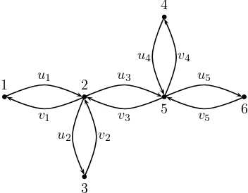
where ei ∼k means that k is an endvertex ofei. Notice that, in view of the Gers-gorin disc theorem, the matrix L is a positive semidefinite matrix. For the sake of convenience, we writewt=ut+vt. Then, the distance matrix Dand the Laplacian matrixLof the bidirected treeT (shown in Figure 2.1) are given by

1 2

5 6

4

3 u1

v1

u3

v3

u5

v5

u2 v2

[image:2.612.168.344.543.680.2]

u4 v4

D= 

      

0 u1 u1+u2 u1+u3+v4 u1+u3 u1+u3+u5

v1 0 u2 u3+v4 u3 u3+u5

v1+v2 v2 0 v2+u3+v4 v2+u3 v2+u3+u5

v1+v3+u4 v3+u4 u2+v3+u4 0 u4 u4+u5

v1+v3 v3 u2+v3 v4 0 u5

v1+v3+v5 v3+v5 u2+v3+v5 v4+v5 v5 0



       ,

and

L= 

       

1

w1 −

1

w1 0 0 0 0

−_w1_{1 w}1₁ +_w1₂ +_w1₃ −_w1₂ −_w1₃ 0 0 0 − 1

w2

1

w2 0 0 0

0 −_w1₃ 0 _w1₄ −_w1₄ 0

0 0 0 −1

w4

1

w3 +

1

w4 +

1

w5 −

1

w5

0 0 0 0 −_w1_{5 w}1₅ 

        .

Observe that if ui =vi = 1 for all i, then the matrices D andL reduce to the matricesD and 1

2L, respectively.

We now introduce some further notation. LetT be a bidirected tree onnvertices. Let ˜T be a spanning tree ofT. Thus, ˜T is obtained fromT by choosing one arc and henceT has 2n−1_{spanning trees. Let us denote theindegreeand theoutdegreeof the}

vertex v in ˜T by In_T˜(v) and Out_T˜(v), respectively. Consider the vectorsz1 andz2

defined by

z1(i) = (−1)n

X

˜

T £

In_T˜(i)−1¤w( ˜T) (2.1)

z2(i) = (−1)n

X

˜

T £

Out_T˜(i)−1¤w( ˜T), (2.2)

wherew( ˜T) is the product of the arc weights of ˜T. For example, the vectorsz1 and z2for the bidirected tree T given in Figure 2.1 are

z1=



       

−u1w2w3w4w5

[−u2u3v1+u1u3v2+u1u2v3+ 2u1v2v3+v1v2v3]w4w5 −v2w1w3w4w5

−u4w1w2w3w5

w1w2[u3u4u5−u5v3v4+ 2u3u4v5+u4v3v5+u3v4v5] −v5w1w2w3w4



and

z2=



       

−v1w2w3w4w5

[u1u2u3+ 2u2u3v1+u3v1v2+u2v1v3−u1v2v3]w4w5 −u2w1w3w4w5

−v4w1w2w3w5

w1w2[u4u5v3+u3u5v4+ 2u5v3v4−u3u4v5+v3v4v5] −u5w1w2w3w4



        .

Note that takingui=vi= 1 for alli, and putting k= InT(i), we see that

(−1)nz1(i) =

X

˜

T £

In_T˜(i)−1¤=

k X

r=0

2n−k−1 X

˜ T

InT˜(i)=r

£

In_T˜(i)−1¤

=h k X

r=0

µ k r ¶

(r−1)i2n−1−k=¡

k2k−1−2k¢

2n−1−k = 2n−2(k−2),

so thatz1=z2= (−1)n−12n−2(e−z).

LetT be a bidirected graph. Since each arc of a spanning tree ˜T contributes 1 to exactly one entry in In_T˜, we have

n P

i=1

In_T˜(i) =n−1.Hence,

zt₁e= n X

i=1

z1(i) =

n X

i=1

(−1)nX

˜

T £

In_T˜(i)−1¤w( ˜T)

= (−1)nX

˜

T w( ˜T)

n X

i=1

£

In_T˜(i)−1¤= (−1)n−1

X

˜

T w( ˜T)

= (−1)n−1 n−1

Y

i=1

wi. (2.3)

A similar reasoning implies that

zt₂e= (−1)n−1

n−1

Y

i=1

wi. (2.4)

For a bidirected treeT onnvertices we definew(T) as

w(T) =X

˜

T

w( ˜T) = n−1

Y

i=1

wi= (−1)n

−1_zt

1e= (−1)n −1_zt

We use the convention that if T is a tree on a single vertex then z1 =e =z2 and

w(T) = 1. With this convention, for a bidirected forestF with the bidirected trees

T1,T2, . . . ,Tk as components, the weight ofF is defined asw(F) = k Q

i=1

w(Ti).

In the next section, we relate the matrices D−1 _{and L and also obtain some}

properties of the matrix D−1 _{with respect to minors. As corollaries, we obtain the}

results of Graham and Pollak [7]) on det(D) and that of Graham and Lovasz [6] on D−1_.

3. The main result. In this section, we extend certain results on distance matrices of trees to distance matrices of bidirected trees. Recall that apendant vertex

is a vertex of degree one. Denote byG−vthe graph obtained by deleting the vertexv and all arcs incident on it fromG. Byek we denote the vector with only one nonzero entry 1 which appears at thekth place.

Given any tree T on vertices {1,2, . . . , n} we may view it as a rooted tree and hence there is a relabeling of the vertices so that for eachi >1 the vertexiis adjacent to only one vertex from {1, . . . , i−1}. With such a labeling the vertexn is always a pendant vertex. Henceforth, unless stated otherwise, each bidirected tree will be assumed to have an underlying tree with such a labeling. Furthermore, fori < j, the weight of an arcej−1 = (i, j) will be assumed to beuj−1 and the weight of the arc

e′

j−1= (j, i) will be assumed to bevj−1. IfT is a bidirected tree byT −ej−1−e′j−1

we denote the bidirected graph obtained by deleting the arcs (i, j) and (j, i) fromT.

We use the method of mathematical induction to prove our results. In the in-duction step, we start with a bidirected treeT′

onk+ 1 vertices, where the pendant vertexk+ 1 is adjacent to the vertexr. We use the definition of the distance matrix of the bidirected tree T = T′

− {k+ 1} to get the distance matrix of T′

. Putting

D′

=D(T′

),D=D(T),L′

=L(T′

),L=L(T), we see that

D′= ·

D uke+Der vket+etrD 0

¸

, L′= "

L+ 1

wkere

t

r −w1ker

−_w1ke

t

r w1k

#

. (3.1)

Furthermore,

(−1)k+1_z′

1(k+ 1) =

X

˜

T £

In_T˜(k+ 1)−1¤w( ˜T)

= X

(k+1,r)∈T˜

[−1]w( ˜T)

Also

(−1)k+1_z′ 1(r) =

X

˜

T £

In_T˜(r)−1¤w( ˜T)

= X

(r,k+1)∈T˜ £

In_T˜(r)−1¤w( ˜T) +

X

(k+1,r)∈T˜ £

In_T˜(r)−1¤w( ˜T)

= (−1)kz1(r)uk + h

(−1)kz1(r)vk+w(T)vk i

,

and fori6=k+ 1, r, we have,

z′₁(i) = (−1)k+1X

˜

T £

In_T˜(i)−1¤w( ˜T)

= (−1)k+1 X

(r,k+1)∈T˜ £

In_T˜(i)−1¤w( ˜T) + (−1)k+1

X

(k+1,r)∈T˜ £

In_T˜(i)−1¤w( ˜T)

=−z1(i)uk −z1(i)vk =−z1(i)wk.

Thus we have

z′₁= ·

−wkz1+ (−1)k+1w(T)vker (−1)k+1_{w(T) (−vk)}

¸

. (3.2)

Similarly we have

z′₂= ·

−wkz2+ (−1)k+1w(T)uker (−1)k+1_{w(T) (−uk)}

¸

. (3.3)

Note that these two equations provide an efficient way of computing the vectorsz1

andz2 for a bidirected tree. Combined with the next theorem they give an efficient

way to compute D−1_{. We shall use our previous observations are in the proof of the}

next theorem.

Theorem 3.1. _{Let D be the distance matrix of a bidirected tree on n vertices}

where the pendant vertexn is adjacent tor. Then

det(D) = (−1)n−1 n−1

X

i=1

uiviw(T −ei−e

′

i) (3.4)

Dz1= det(D)e, z2tD= det(D)et, and (3.5)

D−1_{=−L −(−1)}n z1zt2

Proof. We prove the theorem by induction on the number of vertices of any bidirected tree. So, as the first step, letn= 2. In this case, the matricesD,L,z1 and zt₂are respectively,

D= ·

0 u1

v1 0

¸ , L=

"

1

w1 −

1 w1 − 1 w1 1 w1 #

,z1=−

· u1

v1

¸

, and z2=−

· v1

u1

¸ .

As w(T −e1−e′1) = 1, det(D) =−u1v1 = (−1)2−1u1v1w(T −e1−e′1), Dz1 =

det(D)e and zt

2 D= det(D)et. Thus (3.5) is true forn= 2. Also, for n= 2, the

right hand side of (3.6) reduces to

−L − z1z

t

2

det(D)w(T) =− " ₁

w1 −

1 w1 − 1 w1 1 w1 # − 1

−w1u1v1

·

u1v1 u21

v12 u1v1

¸

=− " ₁

w1 −

1 w1 − 1 w1 1 w1 # + " ₁ w1 u1

v1w1

v1

u1w1

1 w1 # = " 0 1 v1 1

u1 0

# =D−1

Hence (3.6) holds for n= 2. We now assume that the equalities in (3.4), (3.5) and (3.6) are true forn=k. Letn=k+ 1 andT′

be a bidirected tree onk+ 1 vertices. PutT =T′

− {k+ 1}. To establish the first equality (3.5) we need to show that

det(D′) = (−1)k k X

i=1

uiviw(T

′

−ei−e

′

i).

AsDis invertible, using (3.1), the induction hypothesis and (2.3), we have

det(D′) = det(D)£

0−(vket+etrD)D

−1_(u

ke+Der) ¤

(3.7) =−det(D)£

ukvketD−1_e+

vketer+ukerte+etrDer¤

=−det(D)£ ukvk e

t_z

1

det(D)+vk+uk ¤

= (−1)kukvkw(T)−wkdet(D) (3.8)

= (−1)kukvkw(T) + (−1)kwk k−1

X

i=1

uiviw(T −ei−e

′

i)

= (−1)kh_ukvkw(T′

−ek−e′_k) + k−1

X

i=1

uiviw(T′

−ei−e′_i)i

= (−1)k k X

i=1

uiviw(T′−ei−e′i).

To prove the second equality we need to show that

D′z′₁= det(D′)e, z₂′tD′= det(D′)et.

Using the expressions given in (3.1) and (3.2) we have

D′ z′₁=

·

D uke+Der vket+etrD 0

¸ ·

−wkz1+ (−1)k+1w(T)vker (−1)k_w(T)v

k

¸ .

The first block of the vectorD′

z′₁ reduces to

−wkDz1+ (−1)kukvkw(T)e.

Substituting det(D)eforDz1 and using (3.8),

the first block ofD′

z′₁= det(D′

)e. (3.9)

The second block of the vectorD′_z′

1reduces to

−vkwketz1−wketrDz1+ (−1)k+1vkw(T) ¡

vketer+etrDer).

Now using the equalityet

rDer= 0, the equations (2.3), (3.4) and (3.8), we have the second block ofD′z′₁= det(D′). (3.10)

A similar reasoning gives thatz′₂tD′

= det(D′

)et. Hence the second equality is estab-lished forn=k+ 1.

We now prove that the matrixD′−1_{is indeed given by (3.6). As det(D}′_{)6= 0, put}

W = 0−(vket+et_rD)D−1_{(uke+Der). From (3.7), it follows that}

W−1= detD

det(D′₎. (3.11)

Let D′−1

= ·

A11 A12

A21 A22

¸

. Since D′

=

· _D

uke+Der vket+et_rD 0

¸

, it is

straight-forward to see that

A11=D−1+D−1(uke+Der)W−1(vket+etrD)D

−1_{, (3.12)}

A12=−D−1(uke+Der)W

−1_{, (3.13)}

A21=−W−1(vket+etrD)D

−1_{, (3.14)}

A22=W

−1_{. (3.15)}

Using (3.11) and the induction hypothesis, we have

A11=D−1+ detD

det(D′₎

¡ ukD

−1_e+e

r ¢¡

vketD

−1_+et r ¢

=D−1+ detD det(D′₎

µ uk

z1

det(D)+er ¶ µ

vk

zt

2

det(D)+e t r ¶

=D−1+ 1 det(D′₎

· ukvk det(D)z1z

t

2+

¡

ukz1etr+vkerzt2

¢

+ det(D)e_ret_r ¸

and

A12=−D−1(uke+Der)W

−1₌₋ detD

det(D′₎

£ ukD

−1_e+e

r ¤

=−ukz1+ det(D)er

det(D′₎ .

(3.17) Similarly

A21=−

vkzt₂+ det(D)et_r

det(D′₎ . (3.18)

We now determine the first and second blocks of the matrix

−L′

−(−1)k+1 z ′ 1z′2

t

det(D′_)w(T′₎. (3.19)

Using Equations (3.1), (3.2), (3.3), (3.7), (3.11) and the induction hypothesis, the first block of (3.19) equals

−

„

L+ere t r

wk «

+ (−1)k“

w2

kz1zt₂+ukvkw(T)

2

eretr ”

+ukwkw(T)z1etr+vkwkw(T)erzt₂ det(D′₎wkw(T)

=−L+(−1) k_wkz

1zt2

det(D′_)w(T) − eretr

wk

+(−1)

k_ukvkw(T)e retr wkdet(D′)

+ukz1e t

r+vkerzt2

det(D′₎

=D−1₊ (−1)kz1zt2

det(D′_)w(T)

·

wk+det(D

′

) det(D) ¸

−ere

t r wk +

det(D′

) +wkdet(D) wkdet(D′₎ ere

t r

+ukz1e t

r+vkerzt2

det(D′₎

=D−1₊ ukvkz1zt2

det(D′_{) det(D)}+

det(D) det(D′₎ere

t r+

ukz1etr+vkerzt2

det(D′₎ (3.20)

and the second block of (3.19) equals

er wk −

ukwkw(T)z1−(−1)kukvkw(T)2er det(D′_)wkw(T)

= er wk −

ukz1

det(D′₎− er

wkdet(D′₎[det(D ′

) +wkdet(D)]

=−ukz1+ det(D)er

det(D′₎ =−(ukD

−1_e+er)W−1

. (3.21)

Showing thatA21 is the (2,1)-block of (3.19) is similar. The (2,2)-block of (3.19) is

− 1

wk +

(−1)k_u

kvkw(T)2 det(D′_)wkw(T) =−

1 wk +

det(D′

) +wkdet(D) det(D′_)wk =W

−1

.

4. Bidirected trees with two types of weights. SupposeT is a rooted tree with rootr. Letuandv be two vertices ofT. As we traverse theu-vpath fromuto vthere exists a vertex, sayw(which may beuitself), such that the path fromutov moves in the direction ofruntil it meets vertexwand then moves away fromr. Let the lengths of the two pathsu-wandw-v be ℓ1 andℓ2, respectively. Also, letxand

y be two constants. We define the distance betweenuand vas

¯

D(u, v) =ℓ1y+ℓ2x. (4.1)

Clearly, when x =y = 1, this reduces to the usual distance between uand v. We illustrate this with the following example.

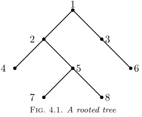
1

2 3

4 5 6

[image:10.612.185.324.297.411.2]

7 8

Fig. 4.1_.A rooted tree

Consider the tree given in Figure 4.1. The distance matrix of the tree is as follows:

¯ D=



           

0 x x 2x 2x 2x 3x 3x

y 0 x+y x x 2x+y 2x 2x

y x+y 0 2x+y 2x+y x 3x+y 3x+y 2y y x+ 2y 0 x+y 2x+ 2y 2x+y 2x+y 2y y x+ 2y x+y 0 2x+ 2y x x 2y x+ 2y y 2x+ 2y 2x+ 2y 0 3x+ 2y 3x+ 2y 3y 2y x+ 3y x+ 2y y 2x+ 3y 0 x+y 3y 2y x+ 3y x+ 2y y 2x+ 3y x+y 0



            .

Observe that if we apply a similar labeling to T as in the previous section and consider the bidirected tree T with the underlying tree structure T, and use the weights ui = x ∀i, vi = y ∀i, then the distance matrix D of the bidirected tree is nothing but the distance matrix ¯D.

Henceforth a rooted tree is assumed to have the root 1 and the labeling as de-scribed earlier. Letube a vertex of a rooted treeT. A vertexvis called achildofuif uand vare adjacent anduis on the v-1 path. Let us denote the number of children ofuby ch(u). With the notations defined above, we have the following result.

matrixD. Also, letz1 andz2 be vectors of ordern given by

(z1)i=

 



(−1)n¡

(ch(i)−1)y−x¢

(x+y)n−2_{, ifi= 1,}

(−1)n−1_y(x+y)n−2_{, ifi is a pendant vertex,}

(−1)n_{(ch(i)−1)y(x+y)}n−2_{, otherwise}

(4.2)

and

(z2)i=

 



(−1)n¡

(ch(i)−1)x−y¢

(x+y)n−2_{, ifi=r,}

(−1)n−1_x(x+y)n−2_{, ifi is a pendant vertex,}

(−1)n_{(ch(i)−1)x(x+y)}n−2_{, otherwise.}

(4.3)

Then

det(D) = (−1)n−1(n−1)xy(x+y)n−2,

and

D−1=− L

x+y +

z1zt2

(n−1)xy(x+y)2n−3,

whereL is the usual Laplacian matrix.

Proof. Let T be the bidirected tree associated withT. As ¯D is the same as D

withui=xandvi=y, the assertion about the determinant follows easily from (3.4).

The vectorsz1,z2 defined here are nothing but the vectors defined in (2.1) and

(2.2). In order to see this note that let ˜T be a spanning tree ofT and putk=ch(1).

(−1)n_z

1(1) =

X

˜

T £

In_T˜(1)−1¤w( ˜T) =

k X

r=0

(x+y)n−1−k X

˜ T

InT˜(1)=r

£

In_T˜(1)−1¤yrxk−r

= (x+y)n−1−k k X

r=0

µ k r ¶

(r−1)yr_xk−r_{= (x+y)}n−1−kh_ky(x+y)k−1_−(x+y)ki

= (x+y)n−2£

(ch(1)−1)y−x¤ .

Ifiis a pendant vertex, putk=ch(i) and observe that

(−1)n_z

1(i) =

X

˜

T £

In_T˜(i)−1¤w( ˜T) =−x(x+y)n−2.

Ifiis any other vertex, then putk=ch(i), and letpbe the parent ofi. We have

(−1)n_z

1(i) =

X

˜

T £

In_T˜(i)−1¤w( ˜T) =

X

(i,p)∈T˜ £

In_T˜(i)−1¤w( ˜T) +

X

(p,i)∈T˜ £

= (x+y) y (k−1)y−x +kxy(x+y) = ch(i)−1 y(x+y) .

The vector z2 may be verified similarly. Now the assertion about inverse of ¯D

follows from (3.6).

As a corollary, we obtain the result of Graham and Pollak [7] on det(D).

Corollary 4.2. _{LetT be a tree onn vertices and letD be its distance matrix.}

Thendet(D) = (−1)n−1_(n−1)2n−2_.

Proof. Let us denote by T the bidirected tree obtained from the given tree T.

As observed earlier, the substitution of ui =vi = 1 for 1 ≤i ≤n−1, reduces the matrixDto the distance matrixD. Under this condition, we havewi=ui+vi= 2 andw(T −ei−e′

i) = 2n

−2 _{for 1≤i≤n−1. Therefore}

det(D_{) = det(}D₎˛ ˛_u

i=vi=1= ( −₁₎n−1

n−1

X

i=1

uiviw(T−ei) ˛ ˛_u

i=vi=1= (

−₁₎n−1₍n−₁₎₂n−2.

We now give a corollary to our result that gives a formula for D−1_{. This result}

was also obtained by Graham and Lovasz (see [6]).

Corollary 4.3. LetT be a tree onn vertices and letD be its distance matrix,

L be its Laplacian matrix and letzandebe the vectors defined earlier. Then

D−1= (e−z)(e−z) t 2(n−1) −

L 2.

Proof. Let us denote by T the bidirected tree obtained from the given tree T.

Observe that under the condition,ui=vi= 1,the matrixDreduces toD, the matrix

Lreduces to L

2 andz1=z2= (−1)

n−2₂n−2_{(z−e). So, we have}

D−1=D−1¯ ¯

ui=vi=1=−L+ (−1)

n−1 z1zt2

det(D)w(T) ¯ ¯

ui=vi=1

=−L

2 +

22n−4_{(e−z)(e−z)}t (n−1)2n−2₂n−1

=−L

2 +

(e−z)(e−z)t 2(n−1) .

REFERENCES

[1] R. B. Bapat, S. J. Kirkland, and M. Neumann. On distance matrices and Laplacians.Linear Algebra Appl., 401:193–209, 2005.

[2] R. B. Bapat, A. K. Lal, and S. Pati. A q-analogue of the distance matrix of a tree.Linear

Algebra Appl.,416:799–814, 2006.

[3] R. B. Bapat and T. E. S. Raghavan.Nonnegative Matrices and Applications.Encyclopedia of Mathematics and its Applications 64, ed. G. C. Rota, Cambridge University Press, Cambridge, 1997.

[4] J. A. Bondy and U. S. R. Murty.Graph Theory with Applications. American Elsevier Publishing Co., New York, 1976.

[5] Miroslav Fiedler. Some inverse problems for elliptic matrices with zero diagonal.Linear Algebra Appl., 332/334:197–204, 2001.

[6] R. L. Graham and L. Lovasz. Distance Matrix Polynomials of Trees.Adv. in Math., 29(1):60–88, 1978.

[7] R. L. Graham and H. O. Pollak. On the addressing problem for loop switching.Bell. System Tech. J., 50:2495–2519, 1971.

[8] F. Harary.Graph Theory. Addison-Wesley, New York, 1969.

[9] L. Hogben. Spectral graph theory and the inverse eigenvalue problem of a graph.Electron. J. Linear Algebra, 14:12—31, 2005.