Derivations of the Moyal Algebra
and Noncommutative Gauge Theories
⋆Jean-Christophe WALLET
Laboratoire de Physique Th´eorique, Bˆat. 210, CNRS, Universit´e Paris-Sud 11, F-91405 Orsay Cedex, France
E-mail: [email protected]
Received October 29, 2008, in final form January 17, 2009; Published online January 30, 2009 doi:10.3842/SIGMA.2009.013
Abstract. The differential calculus based on the derivations of an associative algebra un-derlies most of the noncommutative field theories considered so far. We review the essential properties of this framework and the main features of noncommutative connections in the case of non graded associative unital algebras with involution. We extend this framework to the case ofZ2-graded unital involutive algebras. We show, in the case of the Moyal alge-bra or some related Z2-graded version of it, that the derivation based differential calculus is a suitable framework to construct Yang–Mills–Higgs type models on Moyal (or related) algebras, the covariant coordinates having in particular a natural interpretation as Higgs fields. We also exhibit, in one situation, a link between the renormalisable NC ϕ4-model
with harmonic term and a gauge theory model. Some possible consequences of this are briefly discussed.
Key words: noncommutative geometry; noncommutative gauge theories
2000 Mathematics Subject Classification: 81T75; 81T13
1
Introduction
A class of noncommutative (NC) field theories [1,2] (for general reviews on noncommutative geo-metry, see [3,4]) came under increasing scrutiny after 1998 when it was argued [5,6] that string theory might have effective regimes related to noncommutative field theories (NCFT) defined on a NC version of flat 4-dimensional space. This latter is the Moyal space (see e.g. [7,8]) which has constant commutators between space coordinates. It was further noticed [9, 10] that the simplest NC ϕ4 model, (ϕreal-valued) on the 4-dimensional Moyal space is not renormalisable due to the Ultraviolet/Infrared (UV/IR) mixing [9, 10, 11]. This phenomenon stems from the existence of nonplanar diagrams that are UV finite but nevertheless develop IR singularities which when inserted into higher order diagrams are not of renormalisable type [1,2]. A solution to this problem was proposed in 2004 [12,13]. It amounts to supplement the initial action with a simple harmonic oscillator term leading to a fully renormalisable NCFT (for recent reviews, see e.g. [14, 15]). This result seems to be related to the covariance of the model under the so called Langmann–Szabo duality [16]. Other renormalisable NC matter field theories have then been identified [17,18,19,20] and studies of the properties of their renormalisation group flows have been carried out [21,22,23].
So far, the construction of a renormalisable gauge theory on 4-D Moyal spaces remains a problem. The naive NC version of the Yang–Mills action has UV/IR mixing, which stems from the occurrence of an IR singularity in the polarisation tensor. From a standard one-loop
⋆This paper is a contribution to the Proceedings of the XVIIth International Colloquium on Integrable
calculation, we easily infer that
ωµν(p)∼(D−2)Γ
D
2
˜
pµp˜ν
πD/2(˜p2)D/2 +· · ·, p→0, (1.1)
where ˜pµ≡Θµνpν, Θµν is the symplectic matrix of the 4-D Moyal algebra and Γ(z) denotes the Euler function. This singularity, albeit transverse in the sense of the Slavnov–Taylor–Ward identities, does not correspond to some gauge invariant term. This implies that the recent alter-native solution to the UV/IR mixing proposed for the NCϕ4 model in [24], cannot be extended straighforwardly (if possible at all) to the gauge theories. Note that an attempt to reach this goal has been proposed in [25]. It amounts to add to the naive Yang–Mills action a counterterm which remains invariant under a defined BRST symmetry but however can be viewed as a formal infinite series in the gauge potential Aµ. The actual effect of this counterterm on the UV/IR mixing of the modified gauge action is still unclear and deserves further investigations.
Recently, an extension of the harmonic solution to the case of gauge theories has been pro-posed in [26] and [27] (for various reviews, see [28, 15, 29]). These works have singled out, as potential candidate for renormalisable gauge theory on 4-DMoyal space, the following generic action
S =
Z
d4x
1
4Fµν⋆ Fµν + Ω2
4 {Aµ,Aν}
2
⋆+κAµ⋆Aµ
, (1.2)
where Fµν = ∂µAν −∂νAµ−i[Aµ, Aν]⋆, Aµ is the gauge potential, ⋆ denotes the associative product on the Moyal algebra, [a, b]⋆ ≡ a ⋆ b−b ⋆ a, {a, b}⋆ ≡ a ⋆ b+b ⋆ a and Aµ is the covariant coordinates, a natural gauge covariant tensorial form stemming from the existence of a canonical gauge invariant connection in the present NC framework, as we will recall in a while (see [26, 15]). The 2nd and 3rd terms in (1.2) may be viewed as “gauge counterparts” of the harmonic term of [12]. This action has interesting properties [26,27] deserving further studies. For instance, gauge invariant mass terms for the gauge fields are allowed even in the absence of Higgs mechanism. Besides, the covariant coordinates appear to bear some similarity with Higgs fields. This feature will be examined more closely in the course of the discussion. Unfortunately, the action (1.2) has a non-trivial vacuum which complicates the study of its actual renormalisability [30]. Notice that non trivial vacuum configurations also occur within NC scalar models with harmonic term as shown in [31].
The relevant algebraic framework describing (most of) the classical features of the NC actions considered so far is provided by the differential calculus based on the derivations. This framework has been established in [32,33,34] and [35]. For an exhaustive review, see [36] and references therein. The derivation based differential calculus underlies the first prototypes of NC (matrix-valued) field theories [37,38,39]. For a review, see [40]. As far as the Moyal spaces are concerned, the “minimal” derivation-based differential calculus generated by the “spatial derivations” ∂µ underlies (most of) the works that appeared in the literature, so far. This differential calculus is not unique but can be modified in numerous ways. Among these, a simple modification of the minimal differential calculus has been shown recently to give rise to interesting features [41].
The purpose of this paper is to show that the use of the differential calculus based on the derivations of the Moyal algebra or some related Z2-graded version of it permits one to exhibit interesting features related to gauge theories defined on Moyal space. We show, at least within two non trivial examples, that the derivation based differential calculus is a natural framework to construct Yang–Mills–Higgs type models on Moyal (or related) algebras, the so-called “covariant coordinates” [1, 2] having a natural interpretation as Higgs fields. We also exhibit, in one situation, a link between the renormalisable NC ϕ4-model with harmonic term [12, 13] and
The paper is organised as follows. In Section 2.1 of this paper, we review briefly the main properties of the differential calculus based on the derivations of an associative unital alge-bra and introduce a definition of a NC connection on a module over the algealge-bra, as a natural generalisation of ordinary connections. The specific properties and simplifications occurring when the module is equal to the algebra, which is the case relevant for the NCFT, are detailed in Section 2.2. In Section 2.3, we extend the analysis to Z2-graded algebras. We construct aZ2-graded differential calculus based on the graded derivations of the algebra, set a definition of NC connection, the corresponding curvature and (unitary) gauge transformations. In Sec-tion 3, we focus on the Moyal algebra M. We consider the differential calculus based on the maximal subalgebra of the derivations of M whose elements can be related to (infinitesimal) symplectomorphisms. Then, a direct application of the results of Section 2.2leads to a natural construction of Yang–Mills–Higgs models defined onMwhere the “covariant coordinates” used in the physics literature can be naturally interpreted as Higgs fields, due to the existence of a gauge invariant canonical connection. In Section4we compare in detail the salient mathema-tical features underlying the NC differential calculus of Section 3to those for the NC geometry stemming from the finite dimensional matrix algebraMn(C) as well as for the algebra of matrix valued functions C∞(M)⊗Mn(C). In some sense, the case considered in Section3 interpolates between these two latter situations. The classical properties of the NC Yang–Mills–Higgs actions are also analysed. Explicit one-loop computation of the vacuum polarisation tensor shows that this latter still exhibits an IR singularity of the type given in (1.1). In Section 5 we consider a Z2-graded version of the Moyal algebraMbuilt from two copies of Mand apply the general results derived in Section 2.3 to the construction of a differential calculus generated by a Z2 -graded extension of the derivation algebra considered in Section 3. We show that the gauge theory action built from the “square” of the resulting curvature involves as contributions both the action (1.2) derived in [26] and [27] as well the renormalisable NCϕ4-model with harmonic term elaborated in [12, 13], therefore exhibiting a link between this latter renormalisable NC scalar theory and gauge theories. Finally, a summary of all the main results is presented in Section 6.
2
Dif ferential calculus based on derivations
2.1 General properties
Let A be an associative ∗-algebra with unit I and center Z(A). We denote the involution by
a 7→ a†, ∀a ∈ A. The differential calculus based on the derivations of A is a natural NC generalisation of the usual de Rham differential calculus on a manifold. Basically, the role of the vector fields is now played by the derivations of the algebra. In this subsection, we collect the main properties that will be used in this paper. More details can be found in [32,34,33,35].
Definition 2.1. The vector space of derivations of A is the space of linear maps defined by Der(A) = {X :A → A/ X(ab) = X(a)b+aX(b), ∀a, b ∈ A}. The derivation X ∈ Der(A) is called real if (X(a))†=X(a†),∀a∈A.
The essential properties of the spaces of derivations ofAcan be summarised in the following proposition.
Proposition 2.1. Der(A) is a Z(A)-module for the product (f X)a = f(Xa), ∀f ∈ Z(A),
∀X ∈Der(A) and a Lie algebra for the bracket [X, Y]a=XY a−Y Xa, ∀X, Y ∈Der(A). The
vector subspace of inner derivations is defined by Int(A) ={Ada:b7→[a, b]/ a∈A} ⊂Der(A).
It is a Z(A)-submodule and Lie ideal. The vector subspace of outer derivations is Out(A) = Der(A)/Int(A). The following canonical short exact sequence of Lie algebras and Z(A)-modules
The main features of the differential calculus based on Der(A) are involved in the following proposition. Notice that both the Lie algebra structure and the Z(A)-module structures for Der(A) are used as essential ingredients in the construction.
Proposition 2.2. Let ΩnDer(A) denote the space of Z(A)-multilinear antisymmetric maps from Der(A)ntoA, withΩ0
Der(A) =Aand letΩ•Der(A) =
L
n≥0ΩnDer(A). Then (ΩDer• (A),×,dˆ) is aN -graded differential algebra with the product×onΩ•Der(A)and differentialdˆ: Ωn
Der(A)→ΩnDer+1(A) satisfying dˆ2= 0, respectively defined for∀ω ∈Ωp
Der(A), η∈Ω
q
Der(A) by:
(ω×η)(X1, . . . , Xp+q) = 1
p!q!
X
σ∈Sp+q
(−1)sign(σ)ω(Xσ(1), . . . , Xσ(p))η(Xσ(p+1), . . . , Xσ(p+q)),
ˆ
dω(X1, . . . , Xp+1) =
p+1
X
i=1
(−1)i+1Xiω(X1,· · · ∨i. . . , Xp+1)
+ X
1≤i<j≤p+1
(−1)i+jω([Xi, Xj],· · · ∨i· · · ∨j. . . , Xp+1), (2.1)
where σ denotes permutation and the symbol ∨i indicates that Xi is omitted.
It turns out that a differential calculus can also be built from suitable subalgebras of Der(A). The following proposition holds [32,33]
Proposition 2.3. Let G ⊂ Der(A) denote a Lie subalgebra which is also a Z(A)-submodule.
Then, a restricted derivation-based differential calculus Ω•G(A)can be built fromG. It is obtained
from Proposition 2.2 by replacing the set of ΩnDer(A), ∀n ∈ N by the set of Z(A)-multilinear
antisymmetric maps from Gn to A for n≥0 and still using (2.1).
From now on, we will not write explicitly the product of forms×. It should be obvious from the context when the relevant type of product is used.
In this paper, we will consider a natural NC generalisation of ordinary connections, as intro-duced in [32, 34, 33] to which we refer for more details. It uses left or right finite projective modules on the associative algebra. Notice that alternative NC extensions of connections based on bimodules were considered in [35]. From now on, we denote by M a right A-module. Let
h : M⊗M → A denote a Hermitian structure1 on A. The connection, curvature and gauge transformations are given as follows:
Definition 2.2. A NC connection on M is a linear map∇:M×Der(A)→M satisfying:
∇X(ma) =mX(a) +∇X(m)a, ∇f X(m) =f∇X(m),
∇X+Y(m) =∇X(m) +∇Y(m), (2.2)
∀X, Y ∈Der(A),∀a∈A,∀m∈M,∀f ∈ Z(A). A Hermitian NC connection is a NC connection satisfying in addition X(h(m1, m2)) = h(∇X(m1), m2) +h(m1,∇X(m2)), ∀m1, m2 ∈ M, and
for any real derivation in Der(A). The curvature of ∇ is the linear map F(X, Y) : M → M defined by
F(X, Y)m= [∇X,∇Y]m− ∇[X,Y]m, ∀X, Y ∈Der(A).
Definition 2.3. The gauge group ofMis defined as the group of automorphisms ofMas a right A-module.
1Recall that a Hermitian structure is a sesquilinear map such thath(m
1, m2)† =h(m2, m1), h(ma1, ma2) =
Proposition 2.4. For any g in the gauge group of M and for any NC connection ∇, the
map ∇gX = g−1 ◦ ∇
X ◦g : M → M defines a NC connection. Then, one has F(X, Y)g =
g−1◦F(X, Y)◦g.
It is convenient to require that the gauge transformations are compatible with the Hermitian structure, that is h(g(m1), g(m2)) = h(m1, m2). This defines a NC analogue of unitary gauge
transformations. From now on, we will only consider unitary gauge transformations.
2.2 The free module case
In the special case where M = A, that will be the case of interest for the ensuing discussion, additional simplifications occur. It is further convenient to choose the canonical Hermitian structureh0(a1, a2) =a†1a2.
Proposition 2.5. Assume thatM=Aand h0(a1, a2) =h(a1, a2) =a†
1a2. Then:
i) Any NC connection is entirely determined by ∇X(I) via ∇X(a) =∇X(I)a+X(a), ∀X ∈ Der(A), ∀a ∈ A. The 1-form connection A ∈ Ω1
Der(A) is defined by A : X → A(X) =
∇X(I), ∀X∈Der(A).
ii) Assume that the derivations X are real. Then, a NC connection is Hermitian when
∇X(I)†=−∇X(I).
iii) The gauge group can be identified with the group of unitary elements of A, U(A) and one
has ∇X(I)g =g†∇X(I)g+g†X(g), F(X, Y)g =g†F(X, Y)g, ∀X, Y ∈Der(A), ∀a∈A.
Proof . i) follows directly from Definition2.2(setm=Iin the 1st of (2.2)). Note that the rela-tion ∇X(a) =∇X(I)a+X(a) can be reobtained from the map∇: Ω0Der(A)→Ω1Der(A),∇(a) =
Aa+ ˆda with A :X → A(X) = ∇X(I). For ii), one has (∇X(a1)†a2+a†1∇X(a2)=X(a†1a2) +
a†1(∇X(I)†+∇X(I))a2 where the last equality stems from the expression for ∇X(a) given in i) and the fact thatX is assumed to be real. From this follows ii). Foriii), use Definition2.3and compatibility of gauge transformations with h0 which givesg(a) =g(I)aand h0(g(a1), g(a2)) =
a†1g(I)†g(I)a2 =h0(a1, a2). Then, the gauge transformations for∇X(I) and the curvature stems from Proposition 2.4, the expression for∇X(a) in i) and the expression for F(X, Y).
Definition 2.4. A tensor 1-form is a 1-form having the following gauge transformations:
Ag =g†Ag, ∀g∈ U(A).
There is a special situation where canonical gauge invariant connections can show up, as indicated in the following proposition.
Proposition 2.6. Assume that there exists η ∈ Ω1Der(A), such that daˆ = [η, a], ∀a ∈ A.
Consider the map ∇inv : Ω0
Der(A) → Ω1Der(A), ∇inv(a) = ˆda−ηa, ∀a ∈ A, so that ∇invX (a) =
X(a)−η(X)a. Then, the following properties hold:
i) ∇inv defines a connection which is gauge invariant, called the canonical connection.
ii) For any NC connection ∇, A ≡ ∇ − ∇inv = A+η defines a tensor form. A(X), ∀X ∈
Der(A) are called the covariant coordinates of ∇.
Proof . Since any 1-form can serve as defining a connection in view of Proposition2.5,∇inv(a) =
ˆ
da−ηa is a connection. Notice that it reduces to ∇inv(a) =−aη, since ˆda = [η, a]. Then, one has (∇inv)g(a) =g†∇inv(ga) =g†(d(ga)−ηga) =g†(−gaη) =−aη= ∇inv(a), which shows i).
The property ii) stems simply from Definition 2.4 and the gauge transformations of a NC
The existence of canonical connections translates into some rather general properties of the curvatures, in particular the curvature for the canonical connection. Gauge theories defined on Moyal spaces are a particular example of this, as shown in the next section.
Lemma 2.1. Let Finv(X, Y) ≡ η[X, Y]−[η(X), η(Y)] denote the curvature for the canonical connection. Assume again that there exists η ∈Ω1Der(A), such that daˆ = [η, a], ∀a∈A. Then,
the following properties hold:
i) Finv(X, Y)≡η[X, Y]−[η(X), η(Y)]∈ Z(A).
ii) The curvature of any NC connection defined by the tensor 1-formA can be written as
F(X, Y) = ([A(X),A(Y)]− A[X, Y])−([η(X), η(Y)]−η[X, Y]), ∀X, Y ∈Der(A).
Proof . First, from the definition of ∇inv(a) in Proposition 2.6, one infers that the 2-form curvature associated to the canonical connection is Finv(a) ≡ ∇inv(∇inv(a)) = −( ˆdη−ηη)(a),
∀a∈A. Then, one obtainsFinv(X, Y) =η[X, Y]−[η(X), η(Y)]. Then, from ˆda= [η, a] and ˆd2 = 0, one has ˆd( ˆda) = ˆd(ηa−aη) = [ ˆdη, a]−[η,daˆ ] = [ ˆdη, a]−[η,[η, a]] = [ ˆdη−ηη, a]. From this follows the propertyi). Next, one has∇X(a) =A(X)a−aη(X) so that [∇X,∇Y](a) = [A(X),A(Y)]a−
a[η(X), η(Y)]. ThereforeF(X, Y)(a)=([A(X),A(Y)]−A([X, Y]))a−a([η(X), η(Y)]−η([X, Y])).
This last expression, combined with the property i) implies ii).
Notice that this proposition will be relevant when considering the NC gauge theories on Moyal algebras. A somewhat similar (but not identical!) situation occurs for the algebra of matrices Mn(C) as well as for the algebra of matrix valued functions.
2.3 Graded dif ferential calculus
In this subsection, we extend the previous algebraic scheme to the case of differential calculus based on the derivations of a graded algebra. We consider only the Z2-graded case. The extension to graduations based on additive groups as well as to more general structures [43] will be reported in a separate work [44].
To fix the notations, let A• be a Z2-graded associative unital ∗-algebra, namely A• =
L
α= 0,1Aα where Aα = {a ∈ A•/|a| = α}, |a| denoting the homogeneous degree of a, and
AαAβ ⊆A(α+β)(mod 2). The graded bracket onA• is [a, b]• ≡ab−(−1)|a||b|ba, ∀a, b ∈A•. Let
Z(A•) denote the center of A•, a graded-commutative algebra (a ∈ Z(A•) ⇐⇒ [a, b]• = 0,
∀b∈A•). Graded modules will be needed in the present framework. Recall that they are graded vector spaces M• =L
α=0,1Mα satisfying MαAβ ⊆Mα+β and AβM
α
⊆Mα+β respectively for a right- and left-A•-module.
Definition 2.5. TheZ2-graded vector space of derivations ofA• is Der(A•) =L
α=0,1Derα(A•)
where Derα(A•) is the vector space of linear mapsX of homogeneous degree |X|=α defined by Derα(A•) ={X:Aβ →Aα+β/ X(ab) =X(a)b+ (−1)αβaX(b),∀a∈Aβ,∀b∈A•}.
Most of the properties of the spaces of derivations in the non-graded case can be extended to the graded situation. In the rest of this paper, we will consider the case where the graded module is the graded algebra itself, i.e. M•=A•.
Proposition 2.7. Der(A•) is a graded right Z(A•)-module for the product(zX)(a) =z(X(a)),
a graded left Z(A•)-module for the product (Xz)(a) = (−1)|a||z|(X(a))z, ∀z ∈ Z(A•), ∀X ∈ Der(A•) of homogeneous degree and a Z2-graded Lie algebra of the graded bracket [X, Y]• =
XY −(−1)|X||Y|Y X, ∀X, Y ∈ Der(A•). The Z2-graded vector subspaces of inner derivations
is defined by Int•(A) = {Ada : b 7→ [a, b]•/ a ∈ A•} ⊂ Der•(A). It is a Z2-graded Z(A•)
Proof . The properties follow from straightforward calculations.
Definition 2.6. The space Ωn,αDer(A•), α ∈ {0,1}, n ∈ N denotes the vector space of n-linear maps ω with homogenous degreeα,ω: (Der(A•))×n→A• defined by
i) Ω0Der,α(A•) =Aα,∀α∈ {0,1} and,∀ω∈Ωn,α
Der(A•),∀Xi ∈Der(A•) of homogeneous degree,
ii) ω(X1, . . . , Xn)∈Aα+ Pn
l=1|Xl|,
iii) ω(X1, . . . , Xnz) =ω(X1, . . . , Xn)z,∀z∈ Z(A•), where (Xz) is given in Proposition2.7,
iv) ω(X1, X2, . . . , Xi, Xi+1, . . . , Xn) = (−1)|Xi||Xi+1|ω(X1, X2, . . . , Xi+1, Xi, . . . , Xn).
Proposition 2.8. Let us define ΩDer(A•) =Ln∈N,α=0,1Ω n,α
Der(A•).
Then, the triplet ΩDer(A•),×,dˆ is a bigraded differential algebra with the product × on
ΩDer(A•) and differentialdˆ: Ωn,αDer(A•)→ΩnDer+1,α(A•) such thatdˆ2 = 0 defined by:
i) For any ω∈Ωp,αDer(A•), η∈Ωq,α
Der(A•)
ω×η(X1, X2, . . . , Xp+q)
= 1
p!q!
X
σ∈S(p+q)
(−1)sign(σ)(−1)Pk<l,σ(k)>σ(l)|Xk||Xl|+|η|Pσ(k)≤p|Xk|
×ω(Xσ(1), . . . , Xσ(p))η(Xσ(p+1), . . . , Xσ(p+q)).
ii) The differential is defined, ∀ω∈Ωn,αDer(A•) by:
ˆ
dω(X1, X2, . . . , Xn+1)
= n+1
X
k=1
(−1)k+1(−1)|ω||Xk|(−1)Pkn=1−1|Xk||Xn|X
kω(X1, X2, . . . ,∨k, . . . , Xn+1)
+ X
1≤k<l≤n+1
(−1)k+l(−1)|Xk||Xl|(−1)Pkn=1−1|Xk||Xn|
×(−1)Pln=1−1 |Xl||Xn|ω([X
k, Xl]•, . . . ,∨k,· · · ∨l, . . . , Xn+1),
where the symbol ∨i indicates thatXi is omitted.
iii) A restricted differential calculus is obtained as follows. Let G• ⊂ Der(A•) denote a Z 2 -graded Lie subalgebra andZ(A•)-submodule. A restricted differential calculus based on G•
can be constructed by replacing in i) andii) Der(A•) by G• and eachΩn,α
Der(A•),α∈ {0,1},
n∈Nby the vector space of n-linear mapsω with homogenous degreeα,ω: (G•)×n→A•.
Proof . The proposition can be verified from direct calculation.
As in Section 2.2, we will not write explicitly the symbol × for the product of forms as the product to be used in each case is obvious from the context.
We now define the connection onA• and its curvature as follows:
Definition 2.7. Let Ωn,Der• ≡L
α=0,1Ω
n,α
Der(A•),∀n∈N.
i) The NC connection onA• is defined as a linear map of homogeneous degree 0∇: Ω0,•
Der→
Ω1Der,• such that
∇(a) = ˆda+Aa, ∀a∈A•, A∈Ω1,0
Der(A•),
ii) Let h be a Hermitian structure on A•. The NC connection on A• is Hermitian if it satisfiesX(h(a1, a2)) =h(∇X(a1), a2)+(−1)|X||a1|h(a1,∇X(a2)),∀a1 ∈A•of homogenous
degree |a1|,∀a2 ∈A•, and for any real derivation X in Der(A•) with homogeneous
deg-ree |X|.
iii) The curvature is defined as a linear mapF : Ω0Der,α(A•)→Ω2,α
Der(A•), such that
F(a) =∇(∇(a)) = ( ˆda+AA)(a), ∀a∈A•.
Note that the connection defined here preserves the degree of theZ2-graduation,
∇: Ω0Der,α(A•)→Ω1,α
Der(A•).
Then, one has for any X ∈Der•(A) of homogeneous degree|X|, |A(X)|=|∇X|=|X|. Notice that we do not use a NC analogue of a graded connection. This latter appears to have inter-esting relationship with the concept of superconnection introduced by Quillen [45]. This will be reported elsewhere [46].
From Definition2.7, one obtains the following relations that will be used in the sequel
Proposition 2.9. For any X, Y ∈ Der(A•), any z ∈ Z(A•) and any a ∈A• of homogeneous
degree |X|, |Y|, |z|and |a|, one has
∇X(a) =X(a) +A(X)a; ∇X(ab) =∇X(a)b+ (−1)|X||a|aX(b), ∀b∈A•, (2.3)
∇zX(a) =z∇X(a), ∇Xz(a) = (−1)|a||z|(∇X(a))z, (2.4)
F(X, Y)(a) = ([∇X,∇Y]•− ∇[X,Y]•)(a), ∀a∈A•. (2.5)
Let † denote the involution on A•, (ab)† = (−1)|a||b|b†a† and let h0(a1, a2) = a†
1a2 be the Her-mitian structure on A•. A NC connection on A• as given by Definition 2.7 is Hermitian when
for any real derivation X of homogeneous degree, the 1-form connection A∈ΩDer1,0(A•) satisfies
A(X)†=−A(X).
Proof . The relations (2.3)–(2.5) can be simply obtained from standard calculation. Then, assume that the Hermitian structure is given byh0(a1, a2) =a†1a2 and consider a Hermitian NC
connection ∇. For any real derivation in Der(A•) with homogeneous degree|X|one has, on one hand, X(h0(a1, a2)) =X(a†1)a2 + (−1)|X||a1|a1X(a2) and on the other hand h0(∇X(a1), a2) +
(−1)|X||a1|h
0(a1,∇X(a2)) = (X(a1†) + (−1)|X||a1|a†1A†(X))a2+ (−1)|X||a1|a†1(X(a2) +A(X)a2),
using Proposition 2.9 and the reality ofX. Then, the relation given in Definition2.7
X(h0(a1, a2))A(X) =h0(∇X(a1), a2) + (−1)|X||a1|h0(a1,∇X(a2))
is fulfilled providedA†(X) =−A(X).
The gauge transformations are defined in a way which preserves the degree of the NC con-nection. In the following, we will focus on unitary gauge transformations that are compatible with the Hermitian structure.
Definition 2.8. The gauge group is defined as Aut0(A•), the group of the automorphisms with degree 0 of A•. Let aϕ ≡ ϕ(a) ∀ϕ ∈ Aut0(A•), ∀a ∈ A•. Let h be a Hermitian structure on A•. The unitary gauge group is defined as the subgroup U(A•) ⊂ Aut0(A•) such that
U(A•) ={ϕ∈Aut0(A•)/ h(aϕ
1, a
ϕ
2) =h(a1, a2), ∀a1, a2 ∈A•}.
When h(a1, a2) = h0(a1, a2) = a†1a2, it follows from this definition that the gauge group
Proposition 2.10. For any NC connection ∇ as given in Definition 2.7 and for any ϕ ∈
Aut0(A•), the linear map of homogeneous degree 0 ∇ϕ : Ω0,•
Der → Ω 1,•
Der such that ∇ϕ(a)(X) =
(ϕ−1 ◦ ∇ ◦ϕ)(a)(X), ∀a ∈ A•, ∀X ∈ Der(A•) defines a NC connection. The corresponding 1-form connection is defined by Aϕ=ϕ−1(I) ˆdϕ(I) +ϕ−1(I)Aϕ(I). The gauge transformation of
the curvature is given by Fϕ(a) = (ϕ−1◦F ◦ϕ)(a), ∀a∈A•.
Proof . First, as for iii) of Proposition 2.5, one has aϕ = ϕ(a) = ϕ(I)a, ∀ϕ ∈ Aut0(A•). To
simplify the notations, we setg=ϕ(I). Then, from Definition 2.7, one obtainsϕ−1(∇(ϕ(a))) =
g−1∇(ga) =g−1dˆ(ga) +g−1Aga= ˆda+ (g−1dgˆ +g−1Ag)a. The expression forAϕ follows. The gauge transformation for the curvature can be obtained by a simple calculation.
Proposition 2.6 and Lemma 2.1 must be slightly modified to take into account the total gradingN×Z2. In fact, this can be compactly expressed in terms of differential forms. Note that the bracket on ΩDer(A•) is [ωp, ηq]•=ωη−(−1)pq(−1)|ω||η|ηω,∀ω∈Ωp,Der|ω|(A•),∀η∈Ωq,Der|η|(A•).
The following lemma holds
Lemma 2.2. Assume that ∃η ∈ ΩDer1,0(A•)/daˆ = [η, a]• = ηa−aη, ∀a ∈ A• where dˆis the
differential given in Proposition 2.8. Then, one has the properties:
i) The map ∇inv : Ω0,α
Der(A•) → Ω 1,α
Der(A•), α = 0,1 such that ∇inv(a) = ˆda−ηa = −aη,
∀a ∈ A•, defines a connection in the sense of Definition 2.7. It is called the canonical
connection. ∇inv is gauge invariant: (∇inv)g(a) =∇inv(a), ∀g∈ U(A•).
ii) The curvature for the canonical connection is defined by the linear map Finv: Ω0Der,α(A•)→ Ω2Der,α(A•) such thatFinv(a) = (−dηˆ +ηη)(a),∀a∈A•.
iii) For any NC connection ∇in the sense of Definition 2.7, A ∈ΩDer1,0(A•) such that A(a) = (∇ − ∇inv)(a) = (A+η)(a), ∀a ∈A• defines a tensor form. A(X), ∀X ∈ Der(A•) are
called the covariant coordinates. The curvature for any NC connection ∇is defined by the linear map F : Ω0Der,α(A•)→Ω2,α
Der(A•) such that F(a) =Finv(a) + (AA+ ˆdA −[A, η]•))(a),
∀a∈A•.
iv) For any X, Y ∈ Der(A•), ∀a ∈ A• with respective homogeneous degree |X|, |Y|, |a|, the
following relations hold:
∇invX (a) =−(−1)|X||a|aη(X), ∇X(a) =A(X)a−(−1)|X||a|aη(X), (2.6)
F(X, Y) = [A(X),A(Y)]•− A([X, Y]•) + (η([X, Y]•)−[η(X), η(Y)]•), (2.7)
Finv(X, Y) =−[η(X), η(Y)]•+η([X, Y]•). (2.8)
Proof . From Definition 2.7, any 1-form in Ω1Der,0(A•) defines a connection. In particular, pick
A = −η. The property i) follows. Then, ∀g ∈ U(A•), (∇inv)g(a) =g†∇inv(ga) =−g†(gaη) =
−aη = ∇inv(a). The corresponding curvature is determined by the 2-form F = ˆdA+AA
for A = −η. So, Finv = −dηˆ +ηη. The property for A in iii) is a direct consequence of the definition of a tensor form. The expression forF in terms ofAis obtained by settingA=A−ηin Definition2.7and using the expression forFinv. Finally, the relations given iniv) are obtained by using the main properties of the graded differential calculus given in Proposition2.8. One has in particularAA(X, Y) = [A(X),A(Y)]•, [A, η]•(X, Y) = [η(X),A(Y)]•−(−1)|X||Y|[η(Y),A(X)]•,
ˆ
dA(X, Y) = [η(X),A(Y)]•−(−1)|X||Y|[η(Y),A(X)]•− A([X, Y]•), ˆdη(X, Y) = 2[η(X), η(Y)]•−
η([X, Y]•). Then, the relations (2.6)–(2.8) follow.
elements can be interpreted as infinitesimal symplectomorphisms. This gives rise to a natural construction of Yang–Mills–Higgs type models defined onM. The second case deals with aZ2 -graded differential calculus on aZ2-graded associative algebra built from two copies ofM. Due to the grading, the gauge theory built from the square of the corresponding curvatures involves as contributions the action (1.2) derived in [26] and [27] as well the renormalisable NCϕ4-model
with harmonic term elaborated in [12,13].
From now on, the Hermitian structure ish0(a1, a2) =a†1a2. According to the above discussion,
the gauge group is the group of unitary elements of the associative algebra.
3
Application: gauge theories on the Moyal algebra
3.1 General properties of the Moyal algebra
In this subsection, we collect the properties of the Moyal algebra that will be used in the sequel. For more details, see e.g. [7, 8]). Let S(RD) ≡ S and S′(RD) ≡ S′, with D = 2n, be respectively the space of complex-valued Schwartz functions on RD and the dual space of tempered distributions on RD. The complex conjugation in S, a 7→ a†, ∀a ∈ S, defines a natural involution inS that can be extended toS′ by duality and that will be used in the rest of
this paper. Let Θµν be an invertible constant skew-symmetric matrix which can be written as Θ =θΣ where Σ is the “block-diagonal” matrix, Σ = diag(J, . . . , J) involvingn(2×2) matrixJ
given by J =
0 −1
1 0
and the parameter θ has mass dimension −2. We use the notation
yΘ−1z ≡ y
µΘ−1µνzν. The following proposition summarises properties relevant for the ensuing discussion:
Proposition 3.1. Let the⋆-Moyal product be defined as ⋆:S × S → S by
(a ⋆ b)(x) = 1 (πθ)D
Z
dDydDz a(x+y)b(x+z)e−i2yΘ−1z, ∀a, b∈ S. (3.1)
Then, (S, ⋆) is a non unital associative involutive Fr´echet algebra with faithful trace given by
R
dDx (a ⋆ b)(x) = R
dDx (b ⋆ a)(x) = R
dDxa(x)·b(x), where the symbol “·” is the usual commutative product of functions in S.
The ⋆ product (3.1) can be further extended to S′× S → S′ upon using duality of vector
spaces: hT ⋆ a, bi =hT, a ⋆ bi, ∀T ∈ S′, ∀a, b ∈ S. In a similar way, (3.1) can be extended to
S × S′ → S′, via ha ⋆ T, bi=hT, b ⋆ ai,∀T ∈ S′,∀a, b∈ S. Then, the Moyal algebra is defined
as [7,8].
Definition 3.1. LetMLandMRbe respectively defined byML={T ∈ S′/ a⋆T ∈ S, ∀a∈ S} and MR={T ∈ S′/ T ⋆ a∈ S, ∀a∈ S}. Then, the Moyal algebraMis defined by
M=ML∩ MR.
Notice that ML and MR are sometimes called in the literature respectively the left and right multiplier algebras. By construction,S is a two-sided ideal ofM. The essential structural properties of the Moyal algebra that we will need are summarised in the following proposition:
In the following, we will need the following asymptotic formula for the⋆-product
which holds for any polynomial functions a,b. For a detailed study of the validity of (3.2), see e.g. [47].
Proposition 3.3. The center is Z(M) =C.
Other relevant properties of the⋆-product that hold onMand will be used in the sequel are
Proposition 3.4. For any a, b∈ M, one has the following relations on M:
∂µ(a ⋆ b) =∂µa ⋆ b+a ⋆ ∂µb, (a ⋆ b)†=b†⋆ a†, [xµ, a]⋆=iΘµν∂νa, (3.3a)
Proof . The relations can be obtained by calculations, using from instance the asymptotic
ex-pansion (3.2).
Notice that, as a special case of the last relation (3.3a), one obtains the celebrated relation among the “coordinate functions” defined onM:
[xµ, xν]⋆ =iΘµν, (3.4)
where we set [a, b]⋆ ≡a ⋆ b−b ⋆ a.
As a final remark, note that the Moyal algebra has Z(M) = C as trivial center, which stems from the fact that Θµν is non degenerate. This simplifies the situation regarding all the structures of modules over Z(M) that are involved in the present algebraic scheme. In the present case, these are simply replaced by vector spaces over C.
3.2 Dif ferential calculus and inner derivations
The vector space of derivations ofMis infinite dimensional. Then, a differential calculus based on the full derivation algebra Der(M) would give rise to gauge potentials with an infinite number of components. In view of the construction of physically oriented gauge theories on Moyal spaces, it is more convenient to deal with gauge potentials having a finite number of components. These occur within restricted differential calculi based on Lie subalgebras of Der(A), as given in Proposition 2.3. In the following, we will consider two Lie subalgebras of Der(M), denoted byG1 andG2. The first one is Abelian and is simply related to the “spatial derivatives”∂µ. The resulting differential calculus underlies almost all the constructions of NCFT defined on Moyal spaces. For further convenience, we set from now on
∂µa= [iξµ, a]⋆, ξµ=−Θ−1µνxν, ∀a∈ M. (3.5)
The second derivation Lie subalgebra G2, such that G1 ⊂ G2, is the maximal subalgebra of
Proposition 3.5. Let P2 ⊂ M denote the set of polynomial functions with degree d≤ 2. Let
{a, b}P B ≡Θµν∂x∂aµ∂x∂bν for any polynomial functiona, b∈ M denote the Poisson bracket for the
symplectic structure defined by Θµν. Then, P2 equipped with the Moyal bracket [ , ]⋆ is a Lie
algebra which satisfies
[P1, P2]⋆=i{P1, P2}P B, ∀P1, P2∈ P2.
Proof . Using (3.2), one infers that (P1⋆ P2)(x), ∀P1, P2 ∈ P2 truncate to a finite expansion.
Namely, (P1⋆ P2)(x) =P1(x)·P2(x) +2iΘµν∂P∂xµ1∂x∂Pν2 −14ΘµνΘρσ ∂
2P 1
∂xµ∂xρ
∂P2
∂xν∂xσ where the last term
is a constant. Then, [P1, P2]⋆=iΘµν∂P∂xµ1∂P∂xν2 from which follows the proposition.
Consider now the Lie subalgebraG2 ⊂Der(M) which is the image ofP2 by Ad, G2 ={X ∈
Der(M/ X = AdP, P ∈ P2}. In order to apply Proposition2.6 and Lemma2.1 to the present
situation, one has to define properly the 1-form η from which most of the objects entering the construction of gauge theories are derived. To do this, one defines the linear map η as
η: G2 → P2 / η(X) =P −P(0), ∀X ∈ G2, (3.6)
whereP(0)∈Cis the evaluation of the polynomial functionPatx= 0. Then,X(a) = AdP(a) = Adη(X)(a), ∀X∈ G2,∀a∈ Mand (3.6) can be used to define the 1-form η in the present case.
Notice that η does not define a morphism of Lie algebra since, as implied by the property i) of Lemma2.1, one hasη([X1, X2])−[η(X1), η(X2)]∈Cand is non zero in the present case. Indeed,
take for instanceη(∂µ) =iξµ(see (3.5)); thenη([∂µ, ∂ν])−[η(∂µ), η(∂ν)]⋆= [ξµ, ξν]⋆ =−iΘ−1µν. At this point, some remarks are in order. Proposition 3.5 singles out two subalgebras of derivations, whose elements are related to infinitesimal symplectomorphisms. These are some-times called area-preserving diffeomorphims in the physics literature. The first algebra G1 is
Abelian and is simply the image by Ad of the algebra generated by {Pµ =xµ, µ= 1, . . . , D}, i.e. the polynomials with degree 1. It is the algebra related to the spatial derivatives∂µin view of the 3rd relation of (3.3a) and (3.5). One has immediately, due to (3.4)
[∂µ, ∂ν](a) = [Adiξµ,Adiξν](a) = Ad[iξµ,iξν]⋆(a) = 0, ∀a∈ M.
Note that the interpretation of [xµ, a]⋆ as the Lie derivative along the (constant) Hamiltonian vector fieldiΘµν is obvious. The differential calculus based onG1is the minimal one that can be
set-up on the Moyal algebra and actually underlies most of the studies of the NCFT on Moyal spaces. The second algebra G2 is the image by Ad of {Pµν = (xµxν), µ, ν = 1, . . . , D}, the algebra generated by the polynomials with degree 2. It is the maximal subalgebra of Der(M) whose elements can be related to symplectomorphims. Observe that from (3.3c) and (3.3d) one has
[(xµ·xν), a]⋆=i(xµΘνβ+xνΘµβ)∂βa,
so that the bracket in the LHS can again be interpreted as the Lie derivative along a Hamiltonian vector field. Note that this is no longer true for polynomials with degreed≥3, which is apparent from (3.3e) for d= 3.
OnceG1 orG2 is choose and the corresponding 1-formηis determined, all the properties and
mathematical status of the various objects entering the construction of gauge theories on Moyal spaces are entirely fixed from Proposition 2.6and Lemma2.1. The corresponding relations are summarised below for further convenience. For anyX ∈ Gi,i= 1,2, one has
∇invX (a) =−a ⋆ η(X), A(X) =A(X) +η(X), (3.7)
∇X(a) =∇invX (a) +AX ⋆ a=∇invX (a) + (A(X) +η(X))⋆ a=X(a) +A(X)⋆ a, (3.8)
3.3 Application to the Moyal space
Consider first the Abelian algebra G1 generated by the spatial derivatives (3.5). Then, after
doing a simple rescaling A(X) → −iA(X) (i.e. defining ∇X(I) ≡ −iA(X) so that Hermitian
which fix the respective mathematical status of the objects involved in most of the studies of NCFT on Moyal spaces. The group of (unitary) gauge transformation is the group of unitary elements of M,U(M), as defined in Section 2 and one has
Agµ=g ⋆ Aµ⋆ g†+ig ⋆ ∂µg†, Agµ=g ⋆Aµ⋆ g†,
Fµνg =g ⋆ Fµν⋆ g†, ∀g∈ U(M).
Consider now the algebra G2. Let ¯G2 ⊂ G2 denote the subalgebra of G2 whose image in Mby
the mapη(3.6) corresponds to the monomials of degree 2. The image involves D(D2+1) elements defined by
η(Xµν) =iξµξν ≡η(µν), ∀Xµν ∈G¯2, ∀µ, ν = 1, . . . , D.
The symbol (µν) denotes symmetry under the exchange µ ↔ ν. Notice that the definition forηµν corresponds to real derivations. One has
[η(µν), η(ρσ)]⋆ =− Θ−1ρνη(µσ)+ Θ−1σνη(µρ)+ Θ−1ρµη(νσ)+ Θ−1σµη(νρ)
. (3.10)
which define the generic commutation relations for thesp(2n,R) algebra. Then, the algebra G2 we choose is generated by{∂µ, Xµν}. Its image inMby the mapη(3.6) is the algebraisp(2n,R). One has the additional commutation relations
[ηµ, η(ρσ)]⋆ = Θµρ−1ησ+ Θ−1µσηρ. (3.11)
Notice that any derivation related to isp(2n,R) can be viewed as generating an infinitesimal symplectomorphism, as discussed above. Accordingly, the subalgebra G1 ⊂ G2 can actually be
interpreted physically as corresponding to spatial directions while ¯G2corresponds to (symplectic)
rotations. Notice also that in the caseD= 2, upon defining
therefore making contact with the work carried out in [42]. Note that [42] did not consider the construction of gauge theories on Moyal spaces but was only focused on the construction of subalgebras of the D= 4 Moyal algebra starting from a set of constraints forming a (subal-gebra of a) sp(2n,R) algebra and the obtention of the algebra of smooth functions of R3 from a commutative limit.
A direct application of (3.6), and (3.7)–(3.9) permits one to determine the invariant connec-tion and the tensor form. One obtains
∇inv(∂µ)(a)≡ ∇µinv(a) =−ia ⋆ ξµ, ∇inv(Xµν)(a)≡ ∇inv(µν)(a) =−ia ⋆(ξµξν),
A(∂µ)≡ Aµ=−i(Aµ−ξµ), A(X(µν))≡ A(µν)=−i(A(µν)−ξµξν), (3.12)
where the subscript (µν) denotes symmetry under the exchange of µ and ν. Then, any NC connection is obtained as the sum of the canonical connection and the tensor form, namely
∇µ(a) =∇invµ (a) +Aµ⋆ a=∂µa−iAµ⋆ a,
∇(µν)(a) =∇inv(µν)(a) +A(µν)⋆ a= [iξµξν, a]⋆−iA(µν)⋆ a.
From this, one obtains the following expressions for the curvature
Proposition 3.6. Consider the differential calculus based on the maximal subalgebra of deriva-tions of the Moyal algebra related to symplectomorphisms. The components of the 2-form cur-vature of a NC connection defined by a tensor 1-form with components Aµ,A(µν) are given by
F(∂µ, ∂ν)≡Fµν = [Aµ,Aν]⋆−iΘ−1µν, (3.13)
F(∂µ, X(ρσ))≡Fµ(ρσ)= [Aµ,A(ρσ)]⋆−Θ−1µρAσ−Θ−1µσAρ, (3.14)
F(X(µν), X(ρσ))≡F(µν)(ρσ)= [A(µν),A(ρσ)]⋆+ Θ−1ρνA(µσ)
+ Θ−1σνA(µρ)+ Θ−1ρµA(νσ)+ Θ−1σµA(νρ). (3.15)
Proof . Use Finv(X, Y) ≡ η[X, Y]−[η(X), η(Y)] to evaluate the curvature for the canonical
connection. Consider first Fµνinv. From linearity of η, [∂µ, ∂ν] = 0 and [ηµ, ην] =iΘ−1µν, one finds
Finv
µν = −iΘ−1µν. Then, from (3.9), one gets (3.13). To obtain (3.14), compute [∂µ, X(ρσ)](a) =
[Adηµ,Adη(ρσ)] = Ad[ηµ,ηρσ]⋆ using (3.11). This yields [∂µ, X(ρσ)](a) = Θ
−1
µρ∂σa+ Θ−1µσ∂ρaso that
η([∂µ, X(ρσ)]) = Θ−1µρησ+ Θµσ−1ηρwhich yieldsFµinv(ρσ)= 0. This combined with (3.9) yields (3.14). For (3.15), compute [X(µν), X(ρσ)](a) = Ad[η(µν),η(ρσ)]⋆using (3.10). A straightforward calculation
yieldsF(invµν)(ρσ) = 0. From this follows (3.15).
The gauge transformations are
Agµ=g†⋆ Aµ⋆ g+ig†⋆ ∂µg,
Ag(µν)=g†⋆ A(µν)⋆ g+ig†⋆(ξµ∂ν+ξν∂µ)g, ∀g∈ U(M),
Agµ=g†⋆Aµ⋆ g, Ag(µν)=g†⋆A(µν)⋆ g, ∀g∈ U(M),
Fµνg =g†⋆ Fµν⋆ g, F(gµν)(ρσ)=g†⋆ F(µν)(ρσ)⋆ g, ∀g∈ U(M).
A possible construction of a NC gauge theory defined from the curvature (3.13)–(3.15) can be done as follows. Let [x] denote the mass dimension2 of the quantity x. First, perform the rescalingη(µν)→µθη(µν) whereµis a parameter with [µ] = 1 that will fix the mass scale of the
Higgs field to be identified in a while. Accordingly, the commutation relations (3.10), (3.11) are modified as
[η(µν), η(ρσ)]⋆ =−µθ Θ−1ρνη(µσ)+ Θ−1σνη(µρ)+ Θ−1ρµη(νσ)+ Θ−1σµη(νρ)
,
[ηµ, η(ρσ)]⋆ =µθ Θ−1µρησ+ Θ−1µσηρ
,
and the components of the curvature become
Fµ(ρσ) = [Aµ,A(ρσ)]⋆−µθ Θ−1µρAσ−Θ−1µσAρ,
F(µν)(ρσ) = [A(µν),A(ρσ)]⋆+µθ Θ−1ρνA(µσ)+ Θ−1σνA(µρ)+ Θρµ−1A(νσ)+ Θ−1σµA(νρ)
with (3.13) unchanged. Next, introduce a dimensionfull coupling constant α with mass dimen-sion [α] = 2−n (D = 2n). The functional U(M)-gauge invariant action is then defined by
S(Aµ,A(µν)) =−
1
α2
Z
d2nx Fµν⋆ Fµν+Fµ(ρσ)⋆ Fµ(ρσ)+F(µν)(ρσ)⋆ F(µν)(ρσ)
(3.16)
and is chosen to depend on the fields Aµ and Aµν. The mass dimensions are [Aµ] = [Aµ] = [A(µν)] = 1.
Several remarks are now in order. First, the purely spatial part (3.13) takes the expected form when expressed in term of Aµ through the 1st relation (3.12), namely one obtains easily
Fµν =−i(∂µAν −∂νAµ−i[Aµ, Aν]⋆).
Then, one observes thatFµ(ρσ) can be reexpressed as
Fµ(ρσ) =DAµA(ρσ)−µθ(Θ−1µρAσ−Θ−1µσAρ), DAµA(ρσ)≡∂µA(ρσ)−i[Aµ,A(ρσ)]⋆
using (3.5) and (3.12). DAµA(ρσ) can be interpreted as a “covariant derivative” describing a NC
analogue of the minimal coupling to the covariant fieldAµν. Besides, one has
−α1
Z
d2nxFµ(ρσ)⋆ Fµ(ρσ)=−1
α
Z
d2nx(DAµA(ρσ))2
−4µθ(DµAA(ρσ))Θµσ−1Aσ+ (4n+ 2)µ2AµAµ. (3.17)
In view of the last term in (3.17), the gauge invariant action (3.16) involves a mass term for the gauge potential proportional to∼ (4n+2)α µ2AµAµ. Therefore, bare mass terms forAµcan appear while preserving the gauge invariant of the action. Notice that the translational invariance of the action is broken by the term (4n+ 2)µ2AµAµ in view ofAµ=−i(Aµ−ξµ). Translational invariance is obviously maintened whenever in the action the gauge covariant curvature Fµ(ρσ)
is replaced by the gauge covariant derivative DA µA(ρσ).
The fact thatDA
µA(ρσ)in (3.16) can be viewed as a NC analogue of the covariant derivative of
D(D+1)
2 scalar fieldsAµν, is very reminiscent of a Yang–Mills–Higgs action for which the covariant
4
Discussion
The derivation-based differential calculus is a mathematical algebraic framework that permits one to generate from a given associative algebra different consistent differential calculi. The case of Moyal algebras has been considered in the present paper. Let us compare this latter situation with two other noncommutative geometries, which share some common structures with the one studied here.
First considerMn(C), the finite dimensional algebra ofn×nmatrices. The algebraMn(C) has only inner derivations, a trivial center Cand admits canonical NC gauge invariant connections. This last property is insured by the existence in each case of aC-linear mapη : Der(A)→Asuch that X(a) = [η(X), a] for any a∈ A(A=Mn(C) or M). This map defines a canonical gauge invariant connection on (the right A-module) A: a 7→ ∇Xa = −aη(X). For the differential calculus based on a subalgebra of Der(M), as considered here, the map η is defined by (3.6). For the differential calculus based on Der(Mn(C)), the map is defined by the canonical 1-form connectioniθofMn(C),iθ∈Ω1Der(Mn(C)) interpreted as a map Int(Mn(C))→Mn(C) and such thatiθ(Adγ) =γ−n1T r(γ)I,∀γ ∈Mn(C). However, this last map is a morphism of Lie algebra from Der(Mn(C)) to the subalgebra ofMn(Cformed by the traceless elements (the Lie bracket is the usual commutator) and therefore, the curvature of the canonical connection is zero. This is not the case for the differential calculus considered here. The map η defined in (3.6) is not a Lie algebra morphism which is signaled by a non zero curvature for the canonical connection. Consider now the algebraA=C∞(M)⊗Mn(C) of matrix valued functions on a smooth finite dimensional manifoldM whose derivation-based differential calculus was first considered in [37]. In the present case, Z(A) =C∞(M) and Der(A) = [Der(C∞(M))⊗1]⊕[C∞(M)⊗Der(Mn)] = Γ(M)⊕[C∞(M) ⊗sl
n] in the sense of Lie algebras and C∞(M)-modules. Γ(M) is the Lie algebra of smooth vector fields onM. Then, for any derivationX ∈Der(A),X =X+adγ with
X ∈Γ(M) andγ ∈C∞(M)⊗sln, the traceless elements in A. Set A0=C∞(M)⊗sln. One can identify Int(A) =A0 and Out(A) = Γ(M). Therefore, one has both inner and outer derivations. Finally, one has Ω∗Der(A) = Ω∗(M)⊗Ω∗
Der(Mn) with a differential ˆd = d + d′, where d is the
de Rham differential and d′ is the differential operating on theMn(C) part. The 1-form related to the canonical connection is defined by iθ(X) =γ. As a map from Der(A) to A0, it defines a splitting of Lie algebras andC∞(M)-modules of the short exact sequence
0−→A0−→Der(A)−→Out(A)−→0
while the mapηdefined by (3.6) does not have a similar property. The canonical connection on (the right A-module) Ais defined from −iθ by ∇X(a) = X(a)−iθ(X)a=X(a)−aγ,∀a∈A but is not gauge invariant while the corresponding curvature is zero, due to the above property of splitting of Lie algebras. Past classical studies of the corresponding gauge theories, with an action constructed mainly from the square of the curvature, gave rise to the interpretation of the gauge potential as involving two parts, one being the “ordinary” gauge theories and the other one identifiable as Higgs fields. Indeed, one can show that the simple action ∼ R
dDxFµνFµν constructed using the corresponding curvature Fµν exhibits non trivial vacuum states in the Higgs part, from which a mass generation on the “ordinary” gauge fields is a consequence. This situation has been generalised [38,39] to the case of the algebra of endomorphisms of a SU(n )-vector bundle in the sense that the situation of the trivial bundle correspond to the algebra of matrix-valued functions. Because of the possible non trivial global topology of the bundle, the situation is more involved [38] but reveals essentially that this physical interpretation of the components of the noncommutative gauge fields can be performed in the same way.
The Yang–Mills–Higgs type action constructed from differential calculus based on the subal-gebraG2 ⊂Der(M) in Section3shares common features with this last situation: Each additional
re-lated to an extra noncommutative dimension, corresponds to an additional covariant coordinate that can be interpreted as a Higgs field. Covariant coordinates have thus a natural interpretation as Higgs fields within the framework of the present derivation-based differential calculus. Then, Yang–Mills–Higgs models can be obtained from actions built from the square of the curvature (3.13)–(3.15).
In these type of models, the polarisation tensor for the gauge potentialAµ still exhibits an IR singularity similar to the one given in (1.1) with however a different overall factor depending in particular on the dimension D of the noncommutative space and the Higgs fields content. The calculation can be performed by using auxiliary integrals given below. We consider here the case where no bare mass term for the gauge potential is present. Inclusion of a bare mass term would not alter the conclusion. It is convenient to set Φa ≡ Aµν, a= 1, . . . ,D(D2+1) and The action Scl must be supplemented by a BRST-invariant gauge fixing term SGF, which can be taken as
where the nilpotent Slavnov operationsis defined through the following BRST structure equa-tions
sAµ=∂µC−i[Aµ, C]⋆, sC =iC ⋆ C, sC¯=b, sb= 0,
where λis a real constant andC, ¯C andb denote respectively the ghost, the antighost and the Stuekelberg auxiliary field with ghost number respectively equal to +1, −1 and 0. Recall that
s acts as a graded derivation on the various objects with grading defined by the sum of the degree of differential forms and ghost number (modulo 2). In the following, we will perform the calculation using a Feynman-type gauge. Accordingly, the propagator for the Aµin momentum space takes the diagonal formGµν(p)=δµν/p2. The ghost and Higgs propagators are respectively given by Gg(p)=1/p2 andGHab(p)=2δab/(p2+µ2). The Feynman rules used in the course of the calculation are given in the AppendixA.
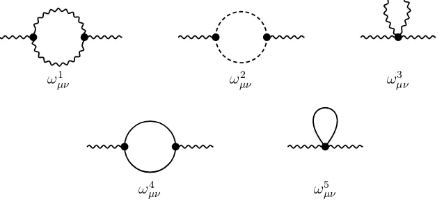
The one-loop diagrams contributing to the vacuum polarisation tensor ωµν(p) are depicted on the Fig. 1. The respective contributions can be written as
ω1
µν ωµ2ν ω3µν
ω4
µν ωµ5ν
Figure 1. One-loop diagrams contributing to the vacuum polarisation tensor. The wavy lines correspond to Aµ. The full (resp. dashed) lines correspond to the Φ (resp. ghost) fields.
It is convenient here to use the Feynman parametrisation, namely ab1 = R1
0 dx(xa+(1−1 x)b)2.
Then, standard manipulations permit one to extract the IR limit of (4.1)–(4.4), denoted by
ωIR
µν(p). In the course of the derivation, it is very convenient to use the following integrals
JN(˜p)≡
Z dDk
(2π)D
eikp˜
(k2+m2)N =aN,DMN−D
2(m|p˜|),
JN,µν(˜p)≡
Z
dDk
(2π)D
kµkνeikp˜
(k2+m2)N =aN,D δµνMN−1−D
2(m|p˜|)−p˜µp˜νMN−2− D
2(m|p˜|)
,
where
aN,D=
2−(D2+N−1)
Γ(N)πD2
, MQ(m|p˜|) = 1
(m2)Q(m|p˜|) QK
Q(m|p˜|)
in which KQ(z) is the modified Bessel function of second kind and of order Q ∈ Z (recall K−Q(z) =KQ(z)) together with the asymptotic expansion
M−Q(m|p˜|)∼2Q−1
Γ(Q) ˜
p2Q , Q >0.
The IR limit of the vacuum polarisation tensor is given by
ωµνIR(p) = (D+N −2)Γ(D 2)
˜
pµp˜ν
πD/2(˜p2)D/2 +· · ·,
where the ellipses denote subleading singular terms. The overall factor affecting ωIR
µν(p) is modified compared to (1.1). It cannot be canceled by tuning the values forDand N. A similar comment applies to ΠIRab(p). Note that a one-loop calculation of the polarisation tensor performed within some N = 1 supersymmetric version of the NC Yang–Mills theory [48] (see also [49]) suggests a better IR behaviour due basically to some compensation occurring between bosonic and fermionic loop contributions.