Full Terms & Conditions of access and use can be found at
http://www.tandfonline.com/action/journalInformation?journalCode=ubes20
Download by: [Universitas Maritim Raja Ali Haji], [UNIVERSITAS MARITIM RAJA ALI HAJI
TANJUNGPINANG, KEPULAUAN RIAU] Date: 11 January 2016, At: 20:33
Journal of Business & Economic Statistics
ISSN: 0735-0015 (Print) 1537-2707 (Online) Journal homepage: http://www.tandfonline.com/loi/ubes20
Adaptive Elastic Net for Generalized Methods of
Moments
Mehmet Caner & Hao Helen Zhang
To cite this article: Mehmet Caner & Hao Helen Zhang (2014) Adaptive Elastic Net for
Generalized Methods of Moments, Journal of Business & Economic Statistics, 32:1, 30-47, DOI: 10.1080/07350015.2013.836104
To link to this article: http://dx.doi.org/10.1080/07350015.2013.836104
Accepted author version posted online: 06 Sep 2013.
Submit your article to this journal
Article views: 403
View related articles
View Crossmark data
Supplementary materials for this article are available online. Please go tohttp://tandfonline.com/r/JBES
Adaptive Elastic Net for Generalized Methods
of Moments
Mehmet C
ANERDepartment of Economics, North Carolina State University, 4168 Nelson Hall, Raleigh, NC 27518 ([email protected])
Hao Helen Z
HANGDepartment of Mathematics, University of Arizona, Tucson, AZ 85718 ([email protected]); Department of Statistics, North Carolina State University, Raleigh, NC 27695 ([email protected])
Model selection and estimation are crucial parts of econometrics. This article introduces a new technique that can simultaneously estimate and select the model in generalized method of moments (GMM) context. The GMM is particularly powerful for analyzing complex datasets such as longitudinal and panel data, and it has wide applications in econometrics. This article extends the least squares based adaptive elastic net estimator by Zou and Zhang to nonlinear equation systems with endogenous variables. The extension is not trivial and involves a new proof technique due to estimators’ lack of closed-form solutions. Compared to Bridge-GMM by Caner, we allow for the number of parameters to diverge to infinity as well as collinearity among a large number of variables; also, the redundant parameters are set to zero via a data-dependent technique. This method has the oracle property, meaning that we can estimate nonzero parameters with their standard limit and the redundant parameters are dropped from the equations simultaneously. Numerical examples are used to illustrate the performance of the new method.
KEY WORDS: GMM; Oracle property; Penalized estimators.
1. INTRODUCTION
One of the most commonly used estimation techniques is the generalized method of moments (GMM) estimation. The GMM provides a unified framework for parameter estimation by encompassing many common estimation methods such as ordinary least squares (OLS), maximum likelihood estimator (MLE), and instrumental variables. We can estimate the param-eters by two-step efficient GMM by Hansen (1982). The GMM is an important tool in econometrics, finance, accounting, and strategic planning literature as well. In this article, we are con-cerned about model selection in GMM when the number of parameters diverges. These situations can arise in labor eco-nomics, international finance (see Alfaro, Kalemli-Ozcan, and Volosovych2008), and so on. In linear models when some of the regressors are correlated with errors and there are a large num-ber of covariates, the model selection tools are essential, since they can improve finite sample performance of the estimators.
Model selection techniques are very useful and widely used in statistics. For example, Tibshirani (1996) proposed the lasso method, Knight and Fu (2000) derived the asymptotic properties of the lasso, and Fan and Li (2001) proposed the SCAD estima-tor. In econometrics, Knight (2008) and Caner (2009) offered Bridge-least squares and Bridge-GMM estimators, respectively. But these procedures all consider finite dimensions and do not take into account the collinearity among variables. Recently, model selection with a large number of parameters has been analyzed in least squares by Huang, Horowitz, and Ma (2008) and Zou and Zhang (2009), where the first article analyzes the Bridge estimator and the second article is concerned with the adaptive elastic net estimator.
Adaptive elastic net estimator has the oracle property when the number of parameters diverges with the sample size.
Fur-thermore, this method can handle the collinearity arising from a large number of regressors when the system is linear with endogenous regressors. When some of the parameters are re-dundant (i.e., when the true model has a sparse representation), this estimator can estimate the zero parameters as exactly zero. In this article, we extend the least squares based adaptive elastic net by Zou and Zhang (2009) to GMM. The following issues are pertinent to model selection in GMM: (i) handling a large number of control variables in the structural equation in a simultaneous equation system, or a large number of pa-rameters in a nonlinear system with endogenous and control variables; (ii) taking into account correlation among variables; and (iii) achieving selection consistency and estimation effi-ciency simultaneously. All of these are successfully addressed in this work. In the least squares case by Zou and Zhang (2009), they do not need an explicit consistency proof since the least squares estimator has a simple and closed-form solution. How-ever, in this article, since the GMM estimator does not have a closed-form solution, an explicit consistency proof is needed before deriving the finite sample risk bounds. This is one ma-jor contribution of this article. Furthermore, to get a consis-tency proof, we have substantially extended the technique used in the consistency proof of Bridge least squares estimator by Huang, Horowitz, and Ma (2008) to the GMM with adaptive elastic net penalty. To derive the finite sample risk bounds, we use the mean value theorem and benefit from consistency proof, unlike the least squares case by Zou and Zhang (2009). The nonlinear nature of the functions introduces additional
© 2014American Statistical Association Journal of Business & Economic Statistics
January 2014, Vol. 32, No. 1
DOI:10.1080/07350015.2013.836104
30
difficulties. The GMM case involves partial derivatives of the sample moments that depend on parameter estimates. This is unlike the least squares case where the same quantity does not depend on parameter estimates. This results in the need for con-sistency proof as mentioned above. Also, we extend the study by Zou and Zhang (2009) to conditionally heteroscedastic data, and this results in tuning parameter forl1norm to be larger than
the one in least squares case. We also pinpoint ways to handle stationary time series cases. The estimator also has the oracle property, and the nonzero coefficients are estimated converging to a normal distribution. This is their standard limit and further-more, the zero parameters are estimated as zero. Note that the oracle property is a pointwise criterion.
Earlier works on diverging parameters include Portnoy (1984), Huber (1988), and He and Shao (2000). In recent years, there are a few works on penalized methods for standard lin-ear regression with diverging parameters. Fan and Peng (2004) studied the nonconcave penalized likelihood with a growing number of nuisance parameters; Lam and Fan (2008) analyzed the profile likelihood ratio inference with a growing number of parameters; and Huang, Horowitz, and Ma (2008) studied asymptotic properties of bridge estimators in sparse linear re-gression models. As far as we know, this is the first article to estimate and select the model in GMM with a diverging num-ber of parameters. In econometrics, sieve estimation will be a natural application of shrinkage estimators. There are several articles that use sieves (e.g., Ai and Chen 2003; Newey and Powell2003; Chen2007; Chen and Ludvigson2009). In these articles, we see that sieve dimension is determined by trying several possibilities or left for future work. Adaptive elastic net GMM can simultaneously determine the sieve dimension and estimate the structural parameters. We also see in unpenalized GMM with many parameters case, there is an article by Han and Phillips (2006). Liao (2011) considered adaptive lasso with fixed number of invalid moment conditions.
Section2 presents the model and the new estimator. Then in Section3, we derive the asymptotic results for the proposed estimator. Section4conducts simulations. Section5 provides an asset pricing example used by Chen and Ludvigson (2009). Section6concludes. The Appendix includes all the proofs.
2. MODEL
Letβ be ap-dimensional parameter vector, whereβ∈Bp, which is a compact subset inRp. The true value ofβisβ
0. We
allowp to grow with the sample sizen, so whenn→ ∞, we havep→ ∞, butp/n→0 asn→ ∞. We do not provide a subscript ofnfor parameter space not to burden ourselves with the notation. The population orthogonality conditions are
E[g(Xi, β0)]=0,
where the data are{Xi :i=1,2. . . , n},g(·) is a known func-tion, and the number of orthogonality restrictions isq,q ≥p. So we also allowqto grow with the sample sizen, butq/n→0 asn→ ∞. From now on, we denoteg(Xi, β) asgi(β) for sim-plicity. Also assume thatgi(β) are independent, and we do not usegni(β) just to simplify the notation.
2.1 The Estimators
We first define the estimators that we use. The estimators that we are interested in aim to answer the following questions. If we have a large number of control variables, some of which may be irrelevant (we may have also a large number of endogenous variables and control variables) in the structural equation in a simultaneous equation system or a large number of parameters in a nonlinear system with endogenous and control variables, can we select the relevant ones as well as estimate the selected system simultaneously? If we have a large number of variables among which there may be possibly some correlation among the variables, can this method handle that? Is it also possible for the estimator to achieve the oracle property? The answers to all three questions are affirmative. First of all, the adaptive elastic net estimator simultaneously selects and estimates the model when there are a large number of parameters/regressors. It can also take into account the possible correlation among the variables. By achieving the oracle property, the nonzero param-eters are estimated with their standard limits, and the zero ones are estimated as exactly zero. This method is computationally easy and uses data-dependent methods to set small coefficient estimates to zero. A subcase of the adaptive elastic net estimator is the adaptive lasso estimator that can handle the first and third questions but does not handle correlation among a large number of variables.
First we introduce the notation: we use the following norms for the vector β1=
p
j=1|βj|, β22=
p
j=1|βj|2, also
β22++ll=p
j=1|βj|2+l, wherel >0 is a positive number. For a matrix A, the norm isA2
2=tr(A′A). We start by
introduc-ing the adaptive elastic net estimator, given the positive and diverging tuning parametersλ1, λ∗1, λ2(how to choose them in
finite samples and its asymptotic properties will be discussed in assumptions and then in the Simulation section):
ˆ
βaenet=(1+λ2/n)
arg min β∈Bp
n
i=1
gi(β)
′
Wn
n
i=1
gi(β)
+λ2β22+λ∗1
p
j=1
ˆ
wj|βj|
⎤
⎦ ⎫ ⎬
⎭
, (1)
where ˆwj =|βˆenet1|γ, ˆβenetis a consistent estimator immediately
explained below,γis a positive constant, andp=nα, 0< α < 1. The assumption onγwill be explained in detail in Assumption 3(iii).Wnis aq×q weight matrix that will be defined in the assumptions below.
The elastic net estimator, which is used in the weights of the penalty above, is
ˆ
βenet=(1+λ2/n)
arg min β∈Bp
Sn(β),
where
Sn(β)=
n
i=1
gi(β)
′
Wn
n
i=1
gi(β)
+λ2β22+λ1β1,
(2)
λ1, λ2are positive and diverging sequences that will be defined
in Assumption 5.
We now discuss the penalty functions in both estimators and explain why we need ˆβenet. The elastic net estimator has both
l1andl2penalties. Thel1penalty is used to perform automatic
variable selection, and the l2 penalty is used to improve the
prediction and handles the collinearity that may arise with a large number of variables. However, the standard elastic net estimator does not provide the oracle property. It turns out that, by introducing an adaptive weight in the elastic net, we can obtain the oracle property. The adaptive weights play crucial roles, since they provide data-dependent penalization.
An important point to remember is when we setλ2 =0 in
the adaptive elastic net estimator (1), we obtain the adaptive lasso estimator. This is simple and we can also get the oracle property. However, with a large number of parameters/variables that may be highly collinear, an additional ridge-type penalty as in adaptive elastic net offers estimation stability and better selection. Before the assumptions we introduce the following notations. Let the collection of nonzero parameters be the set
A= {j :|βj0| =0}and denote the absolute value of the
mini-mum of the nonzero coefficients asη=minj∈A|βj0|. Also, the
cardinality ofAispA(the number of nonzero coefficients). We now provide the main assumptions.
Assumption 1. Define the followingq×pmatrix ˆGn(β)=
n i=1∂gi(β)
∂β′ . Assume the following uniform law of large numbers
sup β∈Bp
Gˆn(β)/n−G(β)22
P
→0,
where G(β) is continuous in β and has a full column rank p. Alsoβ ∈Bp⊂Rp,Bpis compact, and all the absolute value of individual components of the vectorβare uniformly bounded by a constanta,|βj0|,0≤a <∞,j =1, . . . , p. Note that
specif-ically supβ∈Bp
1
n
n
i=1E
∂gi(β)
∂β′ −G(β)
2
2→0, definesG(β).
Assumption 2. Wnis a symmetric, positive definite matrix, andWn−W22
P
→0, whereW is finite and positive definite matrix as well.
Assumption 3.
(i) [n−1n
i=1Egi(β0)gi(β0)′]−1−−122→0.
(ii) Assume p=nα,0< α <1, p/n→0, q/n→0 as
n→ ∞, and p, q→ ∞, q ≥p, so q =nν,0< ν <
1, α≤ν.
(iii) The coefficient on the weights:γ satisfies the following boundγ > 2+α
1−α.
Assumption 4. Assume that
max i
Egi(βA,0)22++ll
nl/2 →0,
for l >0, and where βA,0 represents the true values of the
nonzero parameters and it is ofpAdimension. The dimension also increases with the sample size;pA→ ∞, asn→ ∞, and 0≤pA≤p.
Assumption 5.
(i) λ1/n→0,λ2/n→0,λ∗1/n→0.
(ii)
λ∗
1
n3+αn γ(1−α)
→ ∞. (3)
(iii)
n1−νη2→ ∞. (4) (iv)
n1−αηγ → ∞. (5) (v) Setη=O(n−m), 0< m < α/2.
Now we provide some discussions on the above assumptions. Most of them are standard and used in other papers that estab-lish asymptotic results for penalized estimation in the context of diverging parameters. The rest of them are typically used for the GMM to deal with nonlinear equation systems with endoge-nous variables. Sincep→ ∞, Assumption 1 can be thought of uniform convergence over sieve spacesBp. For the iid subcase, primitive conditions are available in condition 3.5M by Chen (2007).
Assumptions 1 and 2 are standard in the literature of GMM (Chen2007; Newey and Windmeijer2009a,b). They are similar to assumptions 7 and 3 by Newey and Windmeijer (2009a). It is also important to see that Assumption 2 is needed for the two-step nature of the GMM problem. In the first step we can use any consistent estimator (i.e., elastic net) and substitute inWn=n−1
n
i=1gi( ˆβenet)gi( ˆβenet)′in the adaptive elastic net
estimation, where ˆβenet is the elastic net estimator. Also note
that with different estimators, we can define the limit weightW
differently. Depending on the estimatorsWn,Wcan change. As-sumption 3 provides a definition of variance-covariance matrix, and then establishes that the number of diverging parameters cannot exceed the sample size. This is also used by Zou and Zhang (2009). For the penalty exponent in the weight, our con-dition is more stringent than in the least squares case by Zou and Zhang (2009). This is needed for model selection for local to zero coefficients in GMM format. Assumption 4 is a primitive condition for the triangular array central limit theorem. This is also restraining the number of orthogonality conditionsq.
The main issues are the tuning parameter assumptions that reduce bias. We first compare with Bridge estimator by Knight and Fu (2000); there in theorem 3, they needλ/na/2
→λ0≥0,
where 0< a <1, and λ represented the only tuning param-eter. In our Assumption 5(i), we need λ1/n→0, λ∗1/n→
0, λ2/n→0, so ours can be larger than the Knight and Fu
(2000) estimator—we can penalize more in our case. This is due to Bridge type of penalty, which requires less penalization to re-duce bias and get the oracle property. Theorem 2 by Zou (2006) for the adaptive lasso in least squares assumesλ/n1/2
→0. We think the reason that the GMM estimator requires large penal-ization is due to its complex model nature, since there are more elements that contribute to bias here. Theorem 1 by Gao and Huang (2010) display the same tuning analysis as Zou (2006).
The rates onλ1, λ2are standard, but the rate ofλ∗1depends on
αandγ. The conditions onλ1, λ∗1, λ2are needed for consistency
and the bounds on the moments of the estimators. We also allow for local to zero (nonzero) coefficients, but Assumptions 3 and 5 (Equations (4) and (5)) restrict their magnitude. This is tied
to the possible number of nonzero coefficients and seeing that
α≤ν. If there are too many nonzero coefficients (αnear 1), then for model selection purpose the coefficients should slowly approach zero. If there are few nonzero coefficients, to give an example (αnear 0), then the order ofηshould be slightly larger thann−1/2. This also confirms and extends Leeb and P˝otscher (2005) finding that local to zero coefficients should be larger than
n−1/2to be differentiated from zero coefficients. This is shown in proposition A.1(2) in their article. Our results extend that result to the diverging parameter case. Assumption 5(iii) is needed to get consistency for local to zero coefficients. Assumptions 5(iv) and (v) are needed for model selection consistency of local to zero coefficients.
To be specific about implications of Assumptions 5(iii), (iv), and (v) on the order ofη, sinceη=O(n−m), then Assumption 5(iii) implies that
1−ν
2 > m, and Assumption 5(iv) implies that
1−α γ > m.
Combining these two inequalities with Assumption 5(v), we obtain
m <min
1−α γ ,
1−ν
2 ,
α
2
.
Now we can see that with a large number of moments, or a large number of parameters, m may get small, so the magnitude of η should be large. To give an example take
γ =5, α=1/3, ν=2/3, which gives us an upper bound of
m <2/15. So in that scenario,η=O(n−2/15), to get selected as nonzero. It is clear that this is much larger thann−1/2, which Leeb and P˝otscher (2005) found.
Note also that withγ > 21+−αα (i.e., Assumption 3(iii)), we can assure that the conditions onλ∗
1in Assumptions 5(i) and (ii) are
compatible with each other.
Using Assumptions 1, 2, 3(i), we can see that
0< b≤Eigmin[( ˆG(β)′/n)Wn( ˆG(β)/n)], (6)
and
Eigmax[( ˆG(β)′/n)Wn( ˆG(β)/n)]≤B <∞, (7)
with probability approaching 1, where β ∈[β0,βˆw), B >0.
These are obtained by exercise 8.26b by Abadir and Magnus (2005), and lemma A0 by Newey and Windmeijer (2009b) re-sult (eigenvalue inequality for increasing number of dimension case). ˆβw is related to adaptive elastic net estimator and im-mediately defined below. Here Eigmin(M) and Eigmax(M),
re-spectively, represent the minimal and maximal eigenvalue of a generic matrixM.
3. ASYMPTOTICS
We define an estimator that is related to the adaptive elastic net estimator in (1) and also used in the risk bound calculations:
ˆ
βw=arg min β∈Bp
⎡
⎣ n
i=1
gi(β)
′
Wn
n
i=1
gi(β)
+λ2β22
+λ1
p
j=1
ˆ
wj|βj|
⎤
⎦. (8)
The following theorem provides consistency for both the elas-tic net estimator and ˆβw.
Theorem 1. Under Assumptions 1–3 and 5,
(i)
βˆenet−β022
P
→0.
(ii)
βˆw−β022
P
→0.
Remark 1. It is clear from Theorem 1(ii) that adaptive elastic net estimator in (1) is also consistent. We should note that in the article by Zou and Zhang (2009), where the least squares adaptive elastic net estimator is studied, there is no explicit consistency proof. This is due to using a simple linear model. However, for the GMM adaptive elastic net estimator we have the partial derivative ofg(·), which depends on estimators unlike in the linear model case. Specifics are in Equations (A.31)– (A.36). Therefore, we need a new and different consistency proof compared with the least squares case. We need to introduce an estimator that is closely tied to the elastic net estimator above:
ˆ
β(λ2, λ1)=arg min
β∈Bp
Sn(β), (9) whereSn(β) is defined in (2). This is also the estimator we get when we set for allj, ˆwj =1 in ˆβw. Next, we provide bounds for our estimators. These are used then in the proofs for oracle property, and the limits of the estimators.
Theorem 2. Under Assumptions 1–3 and 5,
E
βˆw−β022
≤ 4λ
2
2β022+n 3pB
+λ21Ep
j=1wˆ 2
j+o(n
2
) [n2b
+λ2+o(n2)]2
,
and
Eβˆ(λ2, λ1)−β022
≤4λ
2
2β022+n3pB+λ21p+o(n2)
[n2b+λ
2+o(n2)]2
.
Remark 2. Note that the first bound is related to the estimator in (8), the second bound is related to the estimator in (9), ˆβwis related to the adaptive elastic net estimator in (1), and ˆβ(λ1, λ2)
is related to the estimator in (2). Even thoughβ022=O(p),
andp→ ∞, the bound depends onλ2
2β022/n2→0 in large
samples by Assumptions 3(ii) and 5. Also, λ2 1E
p
j=1wˆj2 is dominated byn4in the denominator in large samples as seen in
the proof of Theorem 3(i). It is clear from the last result that the elastic net estimator is converging at the rate of√n/p.
Theorem 2 extends the least squares case of theorem 3(i) by Zou and Zhang (2009) to the nonlinear GMM case. The risk bounds are different from their case due to the nonlinear nature of our problem. The partial derivative of the sample moment depends on parameter estimates in our case, which complicates the proofs.
Writeβ0 =(βA,′ 0,0′p−pA)
′whereβA,0represents the vector of nonzero parameters (true values). Its dimension grows with the sample size, and 0p−pA vector ofp−pA elements represents
the zero (redundant) parameters. LetβArepresent the nonzero parameters and of dimensionpA×1.
Then define
˜
β =arg min β
⎧ ⎨
⎩ n
i=1
gi(βA)
′
Wn
n
i=1
gi(βA)
+λ2
j∈A
βj2
+λ∗1
j∈A ˆ
wj|βj|
⎫ ⎬
⎭
,
whereA= {j :βj0 =0, j=1,2, . . . , p}. Our next goal is to
show that, with probability 1, [(1+λ2/n) ˜β,0p−pA] converges
to the solution of the adaptive elastic net estimator in (1).
Theorem 3. Given Assumptions 1–3 and 5
(i) with probability tending to 1, ((1+λ2
n) ˜β,0) is the solution to (1).
(ii) (Consistency in Selection) we also have
P({j : ˆβaenet,j =0} =A)→1.
Remark 3. 1. Theorem 3(i) shows that ideal estimator ˜β be-comes the same as the adaptive elastic net estimator in large samples. So the GMM elastic adaptive net estimator has the same solution as ((1+λ2/n) ˜β,0p−pA). Theorem 3(ii) shows
that the nonzero adaptive elastic net estimates display the oracle property with Theorem 4. This is a sharper result than the one in Theorem 3(i). This is an important extension of the least squares case of theorems 3.2 and 3.3 by Zou and Zhang (2009) to the GMM estimation.
2. We allow for local to zero parameters and also provide an assumption when they may be considered as nonzero. This is Assumption 5(iii) and (iv),n1−νη2
→ ∞,n1−αηγ
→ ∞, where
q =nν, p
=nα,0< α
≤ν <1. The implications of the as-sumptions on the magnitude of the smallest nonzero coefficient is discussed after the assumptions. The proof of Theorem 3(ii) clearly shows that, as long as Assumption 5 is satisfied, the model selection for local to zero coefficients is possible. How-ever, the local to zero coefficients cannot be arbitrarily close to zero to be selected. This is well established by Leeb and P˝otscher (2005). Leeb and P˝otscher (2005) showed, in their proposition A1(2), as long as the order of local to zero coefficients is larger thann−1/2in magnitude, they can be selected. So this is like a lower bound for nonzeros to be selected as zeros. Our Assump-tion 5 is the extension of their result to the GMM estimator with a diverging number of parameters. In the diverging pa-rameter case, there is a tradeoff between the number of local
to zero coefficients and the requirement on their order of the magnitude.
Now we provide the limit law for the estimates of the nonzero parameter values (true values). Denote the adaptive elastic net estimators that correspond to nonzero true parameter values as the vector ˆβaenet,A, which is of dimensionpA×1. Define a consistent variance estimator for nonzero parameters that can be derived from elastic net estimators as ˆ∗. We also define−∗1
as[n−1n
i=1Egi(βA,0)gi(βA,0)′]−1−−∗122→0.
Theorem 4. Under Assumptions 1–5, givenWn=ˆ−∗1, set
W =−1
∗ ,
δ′Kn
ˆ
G( ˆβaenet,A)′ˆ∗−1Gˆ( ˆβaenet,A)
1/2
×n−1/2( ˆβaenet,A−βA,0)
d
→N(0,1),
whereKn=[
I+λ2( ˆG( ˆβaenet,A)′ˆ−∗1Gˆ( ˆβaenet,A))−1
1+λ2/n ] is a square matrix of
dimensionpAandδis a vector of Euclidean norm 1.
Remark 4. 1. First we see that
Kn−IpA
2 2
P
→0,
due to Assumptions 1, 2, andλ2=o(n).
2. This theorem clearly extends those by Zou and Zhang (2009) from the least squares case to the GMM estimation. This result generalizes theirs to nonlinear functions of endogenous variables that are heavily used in econometrics and finance. The extension is not straightforward, since the new limit result depends on an explicit separate consistency proof unlike the least squares case by Zou and Zhang (2009). This is mainly because the partial derivative of the sample moment function depends on the parameter estimates, which is not shared by the least squares estimator. The limit that we derive also corresponds to the standard GMM limit by Hansen (1982), where the same result was derived for a fixed number of parameters with a well-specified model. In this way, Theorem 4 also generalizes the result by Hansen (1982) to the direction of a large number of parameters with model selection.
3. Note thatKnterm is a ridge regression like term that helps to handle the collinearity among the variables.
4. Note that if we setλ2=0, we obtain the limit for adaptive
Lasso GMM estimator. In that caseKn=IpA, and
δ′ˆ
G( ˆβalasso,A)′ˆ∗−1Gˆ( ˆβalasso,A) 1/2
n−1/2( ˆβalasso,A−βA,0)
d
→N(0,1).
There will be discussions on how to choose the tuning param-etersλ1, λ2, λ∗1, and how to set the small parameter estimates to
zero in finite samples in the simulation section.
5. Instead of Liapounov central limit theorem, we can use central limit theorem for stationary time series data. These al-ready exist in the book by Davidson (1994). Theorem 4 will proceed as before in the independent data case. When we define the GMM objective function, use sample moments as weighted in time. We conjecture that this results in same proofs for Theo-rems 1–3. This technique of weighting sample moments by time is used by Otsu (2006) and Guggenberger and Smith (2008).
6. After obtaining the adaptive elastic net GMM results, one can run the unpenalized GMM with nonzero parameters and conduct inference.
7. First from Remark 1, we haveKn−IpA
2
2=op(1). Then
δ2=(δ12+ · · · +δ 2
pA)
1/2
=1, andδis apAvector. And then by Assumption 1 and consistency of the adaptive elastic net we haveGˆ( ˆβaenet,A)2=Op(n1/2). These provide the rate of
√
n/pAfor the adaptive elastic net estimators.
4. SIMULATION
In this section we analyze the finite sample properties of the adaptive elastic net estimator for GMM. Namely, we evaluate its bias, the root mean squared error (MSE), as well as the correct number of redundant versus relevant parameters. We have the following simultaneous equations for alli=1, . . . , n
yi =xi′β0+ǫi,
xi =z′iπ+ηi,
ǫi =ρι′ηi+
1−ρ2ι′v i,
where the number of instrumentsq is set to be equal to the number of parametersp,xiis ap×1 vector,ziis ap×1 vector,
ρ=0.5, andπis a square matrix of dimensionp. Furthermore,
ηiis iidN(0, Ip),viis iid withN(0, Ip), andιis ap×1 vector of ones.
The estimated model is:
Eziǫi =0, for alli=1, . . . , n.
We have two different designs for the parameter vectorβ0. In
the first caseβ0= {3,3,0,0,0}(Design 1), and in the second
oneβ0 = {3,3,3,3,0}(Design 2). We haven=100, andzi ∼=
N(0, z) for alli=1, . . . , n, and
z=
⎡
⎢ ⎢ ⎣
1 0.5 0 0 0 0.5 1 0 0 0
0 0 1 0 0
0 0 0 0 1
⎤
⎥ ⎥ ⎦
.
So there is correlation betweenzi’s and this affects the corre-lation betweenxi’s since two equations are correlated. In this section, we compare three methods: GMM-BIC by Andrews and Lu (2001), Bridge-GMM by Caner (2009), and the adaptive elastic net GMM. We use four different measures to compare them here. First, we look at the percentage of correct models selected. Then we evaluate the following summary MSE:
E[( ˆβ−β0)′ǫ( ˆβ−β0)], (10)
whereǫ=Eǫiǫi′, and ˆβ represents the estimated coefficient vector given by three different methods. This measure is com-monly used in statistics literature (see Zou and Zhang2009). The other two measures are concerned about individual coeffi-cients. First, the bias of each individual coefficient estimate is measured. Then the root MSE of each coefficient is computed. We use 10,000 iterations.
Truncation of small coefficient estimates is set to zero via
|βˆBridge|<2/λfor Bridge-GMM as suggested by Caner (2009).
For the adaptive elastic net, we use the modified shooting algo-rithm given in appendix2by Zhang and Lu (2007). Least angle
regression (LAR) is not used because it is not clear whether it is useful in the GMM context.
This modified shooting algorithm amounts to using Kuhn-Tucker conditions for a corner solution. First, the absolute value of the partial derivative of the GMM objective (unpenalized one) with respect to the parameter of interest is evaluated at zero for that parameter, and for the rest at the current adaptive elastic net estimates. If this is less thanλ∗1/|βˆenet|4.5, then we set that
parameter to zero. We have also tried slightly larger exponents than 4.5, and observed that the results are not affected much. Note that the reason for a largeγcomes from Assumption 3(iii). This is similar to the adaptive lasso case used by Zhang and Lu (2007).
The choice of λ’s in both Bridge-GMM and the adaptive elastic net GMM is done via BIC. This is suggested by Zou, Hastie, and Tibshirani (2007) as well as by Wang, Li, and Tsai (2007). Specifically, we use the following BIC by Wang, Li, and Leng (2009). For each pair ofλs=(λ∗1, λ2)∈,
BIC(λs)=log(SSE)+ |A|
log n n ,
where |A| is the cardinality of the set A. SSE=
[n−1n
i=1gi( ˆβ)]′Wn[n−1 n
i=1gi( ˆβ)]. Basically, given a
spe-cificλs, we analyze how many nonzero coefficients are in the estimator and use this to calculate the cardinality ofA, and for that choice compute SSE. The finalλis chosen as
ˆ
λs=arg min λs∈
BIC(λs),
whererepresents a finite number of possible values ofλs. The Bridge-GMM estimator by Caner (2009) is ˆβthat mini-mizesUn(β), where
Un(β)=
n
i=1
gi(β)
′
Wn
n
i=1
gi(β)
+λ
p
j=1
|βj|γ, (11)
for a given positive regularization parameterλand 0< γ <1. We now describe the model selection by GMM-BIC proposed by Andrews and Lu (2001). Letb∈Rp denote a model selec-tion vector. By definiselec-tion, each element ofb is either zero or one. If the jth element ofb is one, the correspondingβj is to be estimated; if the jth element of b is zero we set βj to be zero. We set |b|as the number of parameters to be estimated, or in the equivalent form, |b| =p
j=1|bj|. We then set β[b]
as the p×1 vector representing the element by the element (Hadamard) product of β and b. The model selection will be based on the GMM objective function and a penalty term. The objective function in BIC benefits from
Jn(b)=
n
i=1
gi(β[b])
′
Wn
n
i=1
gi(β[b])
, (12)
where in the simulation
gi(β[b])=zi(yi−xi′β[b]).
The model selection vectors “b” in our case represent 31 dif-ferent possibilities (excluding the all-zero case). The following are the possibilities for all “b” vectors:
M=[M11, M12, M13, M14, M15],
Table 1. Success percentages of selecting the correct model
Estimators Design 1 Design 2
Adaptive Elastic Net 91.2 94.9
Bridge-GMM 100.0 100.0
GMM-BIC 6.9 0.0
NOTE: The GMM-BIC (Andrews and Lu2001) represents the models that are selected according to BIC and subsequently we use GMM. The Bridge-GMM estimator is studied by Caner (2009). The Adaptive Elastic Net estimator is the new procedure proposed in this study.
whereM11is the identity matrix of dimension 5,I5, which
repre-sents all the possibilities with only one nonzero coefficient.M12
represents all the possibilities with two nonzero coefficients,
M12=
⎛
⎜ ⎜ ⎜ ⎜ ⎝
1 1 1 1 0 0 0 0 0 0
1 0 0 0 1 1 1 0 0 0
0 1 0 0 1 0 0 1 1 0
0 0 1 0 0 1 0 1 0 1
0 0 0 1 0 0 1 0 1 1
⎞
⎟ ⎟ ⎟ ⎟ ⎠
. (13)
In the same way, M13 represents all possibilities with three
nonzero coefficients, M14 represents all the possibilities with
four nonzero coefficients, andM15is the vector of ones, showing
all nonzero coefficients. The true model in Design 1 is the first column vector inM12. For Design 2, the true model is inM14
and that is (1,1,1,1,0)′.
The GMM-BIC selects the model based on minimizing the following criterion among the 31 possibilities:
Jn(b)+ |b|log(n). (14) The penalty term penalizes larger models more. Denote the optimal model selection vector by b∗. After selecting the optimal model in (14), the vector b∗, we then estimate the model parameters by the GMM. Next we present the results on Tables1–4for these three techniques that are examined in the simulation section. InTable 1, we provide the correct model se-lection percentages for Designs 1 and 2. We see that both Bridge and Adaptive Elastic Net are doing very well. The Bridge-GMM selects the correct model 100%, and the Adaptive Elastic Net 91%−95% of the time, whereas the GMM-BIC selects only 0%−6.9%. This is due to lots of possibilities in the case of GMM-BIC, and with a large number of parameters the per-formance of GMM-BIC tends to deteriorate.Table 2provides a summary of MSE measure results. This clearly shows that the Adaptive Elastic Net estimator is the best among the three, since its MSE figures are the smallest. The GMM-BIC is much worse in terms of MSE, due to its wrong model selection, and
Table 2. Summary mean squared error (MSE)
Estimators Design 1 Design 2
Adaptive Elastic Net 1.8 1.3
Bridge-GMM 4.2 1.3
GMM-BIC 165848.5 876080.2
NOTE: The MSE formula is given in (10). Instead of expectations, the average of iterations is used. A small number for summary MSE is desirable for a model. The GMM-BIC (Andrews and Lu2001) represents models that are selected according to BIC and subsequently we use GMM. The Bridge-GMM estimator is studied by Caner (2009). The Adaptive Elastic Net is the new procedure proposed in this study.
Table 3. Bias and RMSE results of Design 1
Adaptive
Elastic Net Bridge-GMM GMM-BIC
BIAS RMSE BIAS RMSE BIAS RMSE
β1 −0.244 0.272 −0.117 0.126 2.903 159.85
β2 −0.244 0.272 −0.667 0.669 −4.082 261.32
β3 0.013 0.042 0.000 0.000 −0.859 158.839
β4 0.000 0.009 0.000 0.000 0.612 188.510
β5 0.013 0.041 0.000 0.000 1.162 62.240
NOTE: The GMM-BIC (Andrews and Lu2001) represents models that are selected ac-cording to BIC and subsequently we use GMM. The Bridge-GMM estimator is studied by Caner (2009). The Adaptive Elastic Net estimator is the new procedure proposed in this study.
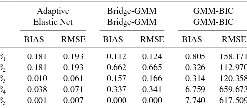
after the model selection estimating the zero coefficients with nonzero and large magnitudes. Tables3and4provide the bias and root MSE of each coefficient in Designs 1 and 2. Compar-ing the Bridge with the Adaptive Elastic Net, we observe that the bias of the nonzero coefficients are generally smaller for the Adaptive Elastic Net. The same is true generally in the case of root MSEs, which are smaller for the nonzero coefficients in the Adaptive Elastic Net estimator.
To get confidence intervals for nonzero parameters, one can run the adaptive elastic net first and find the zero and nonzero coefficients. Then for those nonzero estimates, we have the standard GMM standard errors by Theorem 4. By using that we can calculate confidence intervals for nonzero coefficient parameters.
5. APPLICATION
In this part, we go through a useful application of the new estimator. The following is the external habit specification model considered by Chen and Ludvigson (2009) (also Chen 2007, equation (2.7)):
E
⎛
⎝ι0
C
t+1
Ct
−φ0 1−h0 Ct
Ct+1
−φ0
1−h0
Ct−1
Ct
−φ0Rl,t+1−1|zt
⎞
⎠=0,
whereCt represents the consumption at timet, and ι0 andφ0
are both positive and they represent time discount and curva-ture of the utility function, respectively.Rl,t+1 is thelth asset
Table 4. Bias, RMSE of Design 2
Adaptive Bridge-GMM GMM-BIC Elastic Net Bridge-GMM GMM-BIC
BIAS RMSE BIAS RMSE BIAS RMSE
β1 −0.181 0.193 −0.112 0.124 −0.805 158.171
β2 −0.181 0.193 −0.662 0.665 −0.326 112.970
β3 0.010 0.061 0.157 0.166 −0.314 120.358
β4 −0.038 0.071 0.337 0.341 −6.759 659.673
β5 −0.001 0.007 0.000 0.000 7.740 617.509
NOTE: The GMM-BIC (Andrews and Lu2001) represents models that are selected ac-cording to BIC and subsequently we use GMM. The Bridge-GMM estimator is studied by Caner (2009). The Adaptive Elastic Net estimator is the new procedure proposed in this study.
return at timet+1,h0(.)∈[0,1) is an unknown habit
forma-tion funcforma-tion, andztis the information set and this will be linked to valid instruments. We took only one lag in consumption ra-tio, rather than several of them. The possibility of this specific model is mentioned by Chen and Ludvigson (2009, p. 1069). Chen and Ludvigson (2009) used the sieve estimation to esti-mate the unknownh0 function. They set up the dimension of
the sieve as a given number. In this article, we use the adaptive elastic net GMM to automatically select the dimension of sieve and estimate the structural parameters at the same time. The pa-rameters and the unknown habit function that we try to estimate areδ0, γ0, h0. Now denote
ρ(Ct, Rl,t+1, ι0, φ0, h0)
= ι0
C
t+1
Ct
−φ01−h0 Ct
Ct+1
−φ0
1−h0CCt−1
t
−φ0Rl,t+1−1.
Before setting up the orthogonality restrictions, sets0j(zt) is a sequence of known basis functions that can approximate any square integrable function. Then for each l=1, . . . , N,j =
1, . . . , JT, the restrictions are
E[ρ(Ct, Rl,t+1, ι0, φ0, h0)s0j(zt)]=0.
In total we haveN JTrestrictions, andNis fixed, butJT → ∞, asT → ∞, andN JT/T →0, asT → ∞. The main issue is the approximation of the unknown functionh0. Chen and Ludvigson
(2009) used sieves to approximate that function. In theory the dimension of sieveKT → ∞, butKT/T →0, asT → ∞. Like Chen and Ludvigson (2009), we use an artificial neural network sieve approximation
h
C
t−1
Ct
=ζ0+
KT
j=1
ζj
τj
Ct−1
Ct +
κj
,
where (.) is an activation function, and this is chosen as a logistic function(x)=(1+e−x)−1. This implies that to
es-timate the habit function, we need 3KT +1 parameters. The parameters areζ0, ζj, τj, κj,j =1, . . . , KT. Chen and Ludvig-son (2009) usedKT =3. In our article, along with parameters
δ0, γ0, estimation ofh0 through selection of correct sieve
di-mension will be done. So if true didi-mension of sieve isKT0, with
0≤KT0≤KT, then the Adaptive Elastic Net GMM aims to es-timate that dimension (through estimation of parameters in the habit function). The total number of parameters to be estimated isp=3(KT +1), since we also estimateι0, φ0in addition to the
habit function parameters. The number of orthogonality restric-tions isq =N JT, and we assumeq=N JT ≥3(KT +1)=p. Chen and Ludvigson (2009) used sieve minimum distance timator, and Chen (2007) used sieve GMM estimator to es-timate the parameters. Specifically, equation (2.16) by Chen (2007) uses unpenalized sieve GMM estimation for this prob-lem. Instead we will assume that true dimension of the sieve is unknown and will estimate the parameters along with habit function (parameters in that function) with the adaptive elastic net GMM estimator. Set β =(ι, τ, h) and the compact sieve space isBp =Bδ×Bγ ×HT. The compactness assumption is discussed by Chen and Ludvigson (2009, p. 1067), which is mainly needed so that sieve parameters do not generate tail observations on(.). Also set the approximating known basis
functions ass(zt)=(s0,1(zt), . . . , s0,JT(zt))′, which is aJT×1
vector. SoJT =3, there are three instruments. These are a con-stant, lagged consumption growth, and its square.1 There are seven asset returns that are used in the study, soN =7. The detailed explanations can be found in the article by Chen and Ludvigson (2009).
Implementation Details:
1. First, we run the elastic net GMM to obtain the adaptive weightswj’s. The elastic net GMM has the same objective function as the adaptive version but withwj =1 for all j. The enet-GMM estimator is obtained by setting the weights as 1 in the estimator in the third step given as follows. 2. Then for the weights, since a priori it is known that nonzero
coefficients cannot be large positive, we useγ =2.5 in the exponent. For specifying the weights,wj =1/|βˆenet,j|2.5 is chosen for allj. We have also experimented withγ =4.5 as in the simulations, and the results were mildly different but qualitatively very similar, so those are not reported.
3. Our adaptive elastic net GMM estimator is
ˆ
β =(1+λ2/T) arg min
β∈Bp
⎧ ⎨
⎩ T
t=1
ρ(Ct, Rt+1, β)
$
s(wt)
′
×Wˆ
T
t=1
ρ(Ct, Rt+1, β)
$
s(wt)
+ λ∗1
3(KT+1)
j=1
ˆ
wj|βj| +λ2 3(KT+1)
j=1
βj2
⎫ ⎬
⎭
,
where β1=ι,β2=φ, and the remaining 3KT +1 param-eters correspond to the habit function estimation by sieves. We use the following weight to make the comparison with Chen and Ludvigson (2009) in a fair way:
ˆ
W =I⊗(S′S)−,
whereSis (s(z1), . . . , s(zt), . . . , s(zT))′, which isT ×3 ma-trix, where we use Moore-Penrose inverse as described in (2.16) by Chen (2007). Note thatρ(Ct, Rl,t+1, β) is anN×1
vector, and
ρ(Ct, Rt+1, β)=(ρ(Ct, R1,t+1, β), . . . ,
ρ(Ct, Rl,t+1, β), . . . , ρ(Ct, RN,t+1, β))′.
After the implementation steps we explain the data here. The data points start from the second quarter of 1953 and end at the second quarter of 2001. This is a slightly shorter span than Chen and Ludvigson (2009) since we did not want to use missing data cells for certain variables. SoN JT =21 (number of orthogonal-ity restrictions). At first we tryKT =3 like Chen and Ludvigson (2009), but this is the maximal number of sieve dimension, and we estimate sieve parameter with structural parameters and se-lect the model unlike Chen and Ludvigson (2009). We also try
KT =5. WhenKT =3, the total number of parameters to be
1There are more instruments that are used by Chen and Ludvigson (2009), but
only these three are available to us. Also we thank Sydney Ludvigson to remind us the discrepancy in the unused instruments in her website and theJournal of Applied Econometricswebsite.
estimated is 12, and if KT =5, then this number is 18. We also use BIC to choose from three possible tuning parameter choices,λ1=λ∗1 =λ2= {0.000001,1,10}. The tuning
param-eters are taking the same value for ease of computation. So here we will compare our results with unpenalized sieve GMM by Chen (2007). As discussed above we apply a certain sub-set of the instruments, since the remainder are unavailable, and do not use missing data in the article by Chen and Ludvig-son (2009). So our results corresponding to unpenalized sieve GMM will be slightly different than that by Chen and Ludvigson (2009).
We provide the estimates for our adaptive elastic net GMM method. This is for the case of KT =5. The time discount estimate ˆι=0.88 and the curvature of the utility curve pa-rameter is ˆφ=0.66. The sieve parameter estimates are ˆζ0=0,
ˆ
ζj =0,0,0,0,0, ˆτj =0.086,0.078,0.084,0.073,0.083, ˆκj = 0.082,0.072,0.087,0.086,0.080, forj =1,2,3,4,5, respec-tively. To compare if we use sieve GMM with imposingKT =5 as the true dimension of the sieve, we get ˆιsg=0.86 and ˆφsg= 0.73 for time discount and curvature parameter, where subscript
sgdenotes Chen and Ludvigson (2009) and Chen (2007) with
λ1 =λ∗1 =λ2=0. So the results are basically the same as ours
for these two parameters. However, the estimates of sieve param-eters in unpenalized sieve GMM case is ˆζsg,0=0, ˆζsg,j =0 for allj =1, . . . ,5, and ˆτsg,j =0.083,0.079,0.079,0.079,0.076,
ˆ
κsg,j =0.089,0.086,0.086,0.084,0.082, respectively, forj = 1, . . . ,5. So the habit function in the sieve GMM withKT =5 is estimated as zero (on the boundary); our method gives the same result.
Chen and Ludvigson (2009) fit KT =3 for the sieve. We provide the estimates for our adaptive elastic net GMM method in this case as well. We also reestimate Chen and Ludvig-son (2009). In the adaptive elastic net GMM, the time dis-count estimate is ˆι=0.93 and the curvature of the utility curve parameter is ˆφ=0.64. The sieve parameter estimates are ˆζ0=0, ˆζj =0, for j =1,2,3 ˆτj =0.057,0.054,0.064,
ˆ
κj =0.067,0.066,0.058, forj =1,2,3,respectively. To com-pare with our method we use the sieve GMM by Chen and Lud-vigson (2009) with imposingKT =3 as the true dimension of the sieve, and get ˆιsg=0.94 and ˆφsg=0.71 for time discount and curvature parameter, where subscriptsgdenotes Chen and Ludvigson (2009) and Chen (2007) withλ1=λ∗1=λ2 =0. So
the results are again basically the same as ours for these two pa-rameters. However, the estimates of sieve parameters in unpenal-ized sieve GMM case is ˆζsg,0=0, ˆζsg,j =0.022,0.025,0.019 for all j =1, . . . ,3, and ˆτsg,j =0.051,0.055,0.056, ˆκsg,j = 0.076,0.075,0.075, respectively, forj =1, . . . ,3. So the habit function in the adaptive elastic net GMM withKT =3 is esti-mated as zero (on the boundary), but with the sieve GMM, the estimate of the habit function is positive. Chen and Ludvigson (2009), with a larger instrument set than we used for their case, find the time parameter estimate to be 0.99 and curvature to be 0.76, and the habit function was positive atKT =3. Note that we use time series data, and as we suggest after our theorems, this is plausible given our technique and the structure of the proofs.
We now discuss how our assumptions fit this application. First, all of our parameters are uniformly bounded in this
ap-plication, which is discussed by Chen and Ludvigson (2009, p. 1067). Then the second issue is whether the uniform conver-gence of partial derivative is plausible. This will be satisfied in iid case through condition 3.5M by Chen (2007). This amounts to uniformly bounded partial derivatives, Lipschitz continuity of partial derivatives, and log of covering numbers to be growing less than rateT.
Assumption 2 is related to convergence of the weight matrix, which is not restrictive, and it shows a relation betweenqandT, soqcannot grow fast. In our caseq=N JT, whereNis fixed, so this restricts the growth ofJT. Assumption 3(i) is also similar to Assumption 2. For Assumption 3(ii), we havep=3(KT + 1), since q=N JT ≥3(KT+1)=p, given that N JT/T → 0 provides us the assumption. Assumption 3(iii) is satisfied here by imposing a value between 0 and 1 (including one) for the exponent in the elastic net based weights. Assumption 4 is concerned about the sample moment functions, since all of our variables are stationary, in terms of ratios, and bounded variables such as returns; we do not expect its 2+lmoment to grow larger thanT1/2. Assumption 5 is a penalty function, and this is satisfied with usingTin place ofn.
6. CONCLUSION
In the article here we analyze the adaptive elastic net GMM estimator. It can simultaneously select the model and estimate that. The new estimator also allows for a diverging number of parameters. The estimator is shown to have the oracle property, so we can estimate nonzero parameters with the standard GMM limit and the redundant parameters are set to zero by a data-dependent technique. Commonly used AIC, BIC methods as well as our estimator face some nonuniform consistency issues of the estimators. If we have to select the model with AIC or BIC and then use GMM, this also has the nonuniform consis-tency issues and also does much worse than the adaptive elastic net estimator considered here. The issue with model selection (i.e., including AIC, BIC) is that all of them are uniformly in-consistent (from model selection perspective). So any arbitrarily local to zero coefficients cannot be selected as nonzero. Leeb and P˝otscher (2005) established that, to get selected, the order of the magnitude of local to zero coefficients should be larger thann−1/2. Between 0 and the magnitude ofn−1/2, the model selection is indeterminate. We study the selection issue of local to zero coefficients in the GMM and extend the results by Leeb and P˝otscher (2005) to the GMM with a diverging number of parameters.
APPENDIX
Proof of Theorem 1(i). Huang, Horowitz, and Ma (2008) an-alyzed the least squares with Bridge penalty with a diverging number of parameters. Here we extend that to a diverging num-ber of moment conditions with parameters and the Adaptive Elastic Net penalty in nonlinear GMM.
Starting with ˆβenetdefinition
(1+λ2/n)Sn( ˆβenet)≤(1+λ2/n)Sn(β0),
which is
which is aq×pmatrix. The next two equations ((A.4)– (A.6)) are from the article by Huang, Horowitz, and Ma (2008, p. 603). We use them to illustrate our point. Then it is clear that (A.3) can be written as
′nn−2Dn′n−ιn≤0, (A.4) which provides us
n−Dn22− Dn22−ιn≤0. Using the last inequality, we deduct
n−Dn2≤ Dn2+ι1n/2, and by triangle inequality
n2≤ n−Dn2+ Dn2≤2Dn2+ι1n/2. (A.5) By using (A.4) and (A.5) with simple algebra, we have
n22≤6Dn22+3ιn. (A.6)
with probability approaching 1, by substitutingW =−1
and by Assumptions 2 and 3. Then by the definition ofDnand (A.4)
EDn22−nE
Using (A.8) in (A.7) with the definition ofDn, with probability approaching 1,
ED2n22=O(nq). (A.9) Next by the definition ofnand Assumption 2, we have
n22 =n
with probability approaching 1 and seeing (6) with remembering that elastic net is a subcase of ˆβw. Next use (A.9) and (A.10) in (A.6) to have
n2bEβˆenet−β022≤O(nq)+O(λ1pA+λ2pA), (A.11)
by seeing that λ1j∈A|βj0| +λ2j∈Aβj20 =O(λ1pA+
λ2pA), given that nonzero parameters can be all constants at
most. So by Assumptions 3 and 5, sinceλ1/n→0, λ2/n→0,
Proof of Theorem 1(ii). The proof for the consistency of the estimator ˆβw is the same as in the elastic net case in Theorem 1(i). The only difference is the definition of ιn=
λ1
only nonzero coefficient weights play a role in termιn. As in (A.11)
The key issue is the order of the penalty terms. We are only interested in nonzero parameter weights. Defining
ˆ
η=minj∈A|βˆj,enet|, we have forj ∈A,
ˆ
wj = 1
|βˆj,enet|γ
≤ 1
ˆ
ηγ. Then
λ1j∈Awˆj|βj0|
n2 ≤
λ1ηˆ−γpAC
n2 , (A.13)
where we use maxj∈A|βj0| ≤C, whereCis a generic positive
constant. So we can write (A.13)
λ1ηˆ−γpAC
n2 =
'λ
1η−γpAC
n2
&
ˆ
η η
−γ
. (A.14) In the above equation we first show
E
ˆ
η η
2
=O(1). (A.15)
First see that by simple algebraic inequality as in (6.13) by Zou and Zhang (2009),
E
ˆ
η η
2
≤2+η22E( ˆη−η) 2
≤2+η22Eβˆenet−β0 2
2. (A.16)
Next by Theorem 1(i) (Equation (A.11))
1
η2Eβˆenet−β0 2 2=O
qn
+λ1pA+λ2pA
n2η2
,
sinceλ1/n→0, λ2/n→0, andpA≤q, the largest stochastic order is qn/n2η2
=q/nη2. By q
=nν, and 0< ν <1 with
n1−νη2
→ ∞by Assumption 5(iii) clearly 1
η2Eβˆenet−β0 2
2=o(1). (A.17)
Next by (A.16) and (A.17) we have
E
ˆ
η η
2
≤2+o(1).
So (A.15) is shown, and by Markov’s inequality
ˆ
η η
2
=Op(1),
clearly (ηηˆ)2
=op(1). Note that
ˆ
η η
−γ
=
ˆ
η η
2−γ /2
. (A.18)
Then by (A.18) we have
ˆ
η η
−γ
=Op(1). Next on the right-hand side of (A.14)
λ1
n pAC
nηγ →0,
sinceλ1/n→0 by Assumption 5(i), and by Assumption 5(iv)
n1−αηγ
→ ∞. The last two equations illustrate that (A.14)
λ1ηˆ−γpAC
n2 =
'λ
1η−γpAC
n2
&
ˆ
η η
−γ
P
→0. (A.19) Next in (A.12) we have
λ2j∈Aβ
2
j0
n2 =O
λ
2pA
n2
=o(1), (A.20) byλ2/n→0,pA/n→0. Also note that byq/n→0 through Assumption 3 combining (A.19) and (A.20) in (A.12) above provides us
Eβˆw−β022
= O(nq n2
)
+O
λ1j∈Awˆj|βj0| +λ2j∈Aβj20
n2
= o(1). (A.21)
Proof of Theorem 2. In this proof we start by analyzing the GMM-Ridge estimator that is defined as follows:
ˆ
βR=arg min β
n
i=1
gi(β)
′
Wn
n
i=1
gi(β)
+λ2β22.
Note that this estimator is similar to the elastic net estimator, if we setλ1=0, in elastic net estimator, then we obtain the
GMM-Ridge estimator. So since the elastic net estimator is consistent, GMM-Ridge will be consistent as well. Define also the followingq×pmatrix ˆGn( ˆβR)=
n i=1∂gi( ˆβR)
∂β′ . Then set ¯β ∈
(β0,βˆR). Note that ˆGn( ¯β) is the value of ˆGn(.) evaluated at ¯β. A
mean value theorem aroundβ0applied to first-order conditions
provides, withgn(β0)=in=1gi(β0),
ˆ
βR = −[ ˆGn( ˆβR)′WnGˆn( ¯β)+λ2Ip]−1
×[ ˆGn( ˆβR)′Wngn(β0)−Gˆn( ˆβR)′WnGˆn( ¯β)β0]. (A.22)
Also using the mean value theorem with first-order condi-tions, adding and subtractingλ2β0 from first-order conditions
yields
ˆ
βR−β0 = −[ ˆGn( ˆβR)′WnGˆn( ¯β)+λ2Ip]−1
×[ ˆGn( ˆβR)′Wngn(β0)+λ2β0]. (A.23)
We need the following expressions by using (A.22)
ˆ
βR′[ ˆGn( ˆβR)′Wngn(β0)−Gˆn( ˆβR)′WnGˆn( ¯β)β0]
= −[ ˆGn( ˆβR)′Wngn(β0)−Gˆn( ˆβR)′WnGˆn( ¯β)β0]′
×[ ˆGn( ˆβR)′WnGˆn( ¯β)+λ2Ip]−1
×[ ˆGn( ˆβR)′Wngn(β0)−Gˆn( ˆβR)′WnGˆn( ¯β)β0] (A.24)
ˆ
βR′[ ˆGn( ˆβR)′WnGˆn( ¯β)+λ2Ip] ˆβR
= [ ˆGn( ˆβR)′Wngn(β0)−Gˆn( ˆβR)′WnGˆn( ¯β)β0]′
×[ ˆGn( ˆβR)′WnGˆn( ¯β)+λ2Ip]−1
×[ ˆGn( ˆβR)′Wngn(β0)−Gˆn( ˆβR)′WnGˆn( ¯β)β0]. (A.25)
Next the aim is to rewrite the following GMM-Ridge objective function via a mean value expansion
n Then use Assumption 1 to have
ˆ where the oP(1) term comes from the uniform law of large numbers. Clearly the stochastic order of the second term is smaller than the first one on the right-hand side of (A.27). By using the same argument to get (A.27), we have
ˆ
Again the second term’s stochastic order is smaller than the first one in (A.28).
Furthermore we can rewrite the right-hand side of (A.26)
gn(β0)′Wngn(β0)
whereso1represents the small-order terms mentioned in (A.27)
and (A.28). The equality is obtained through (A.24) and (A.25) via Assumption 1 and the consistency of GMM-Ridge since
ridge is a subcase of elastic net with λ1=0 imposed on the
elastic net. Note that the right-hand side expression in (A.24) is just the negative of the right-hand side of the expression in (A.25). As in (A.29), for the estimator ˆβwwe have the following where ¯βw∈(β0,βˆw), The termso2above comes from the same type of analysis done
for the second and small stochastic order terms in (A.27) and (A.28). Next substitute (A.31) into (A.30) to have
n
approximation error between ¯β and ¯βw. Specifically note that ˆ
β′
wso2βˆR βˆR′so3βˆw βˆw′so4βˆw are smaller-order terms than the second, third, and fourth terms on the right-hand side of (A.32), respectively. Denote so5=min(so1, so2, so3, so4). Now
sub-tract (A.29) from (A.32) to have
n The next analysis is very similar to equations (6.1)–(6.6) by Zou and Zhang (2009). After this important result see that by
the definitions of ˆβwand ˆβR Then also see that
p
Next benefit from (A.34), with (A.33) and (A.35) to have
( ˆβw−βˆR)′[ ˆGn( ¯β)′WnGˆn( ¯β)+λ2Ip]( ˆβw−βˆR) order than so5, which is explained in (A.32) and (A.29). We
also want to modify the last inequality. By the consistency of ˆ
βw,βˆR, ¯β P
→β0. Then with the uniform law of large numbers
on the partial derivative we have by Assumptions 1–3
.
Using lemma A0 by Newey and Windmeijer (2009b), modify (A.37) in the following way given the last equality, setW =−1
(since this is the efficient limit weight as shown by Hansen (1982))
Now we consider the second part of the proof of this theorem. We use the GMM ridge formula. Note that from (A.23)
ˆ
βR−β0= −λ2[ ˆGn( ˆβR)′WnGˆn( ¯β)+λ2Ip]−1β0
−[ ˆGn( ˆβR)′WnGˆn( ¯β)+λ2Ip]−1[ ˆGn( ˆβR)′Wngn(β0)].
(A.40)
We try to modify the above equation a little.
In the same way we obtain (A.38)
Gˆn( ˆβR)′Wngn(β0)−n[G(β0)′W gn(β0)]−oP(n)22
where the last inequality is by (A.42). Note that we do not use orders smaller thano(n2) in (A.44) since this will not make any difference in the proofs of the theorems below. Now use (A.39) and (A.44) to have
Eβˆw−β022
Proof of Theorem 3(i). The proof is similar to proof of the-orem 3.2 by Zou and Zhang (2009). The differences are due to nonlinear nature of the problem. Our upper bounds in Theorem 2 converge to zero at a different rate than Zou and Zhang (2009). To prove the theorem, we need to show the following (Note that by Kuhn-Tucker conditions of (1)),
P derivative matrix that corresponds to irrelevant parameters,
evaluated at ˜β. Or we need to show
Then as in equation (6.7) by Zou and Zhang (2009), we can show that
where the second inequality is due to Theorem 2. Then we can also have
converges to zero faster.
In (A.48) we consider the second term on the right-hand side. Via inequality (6.8) by Zou and Zhang (2009) and Theorem 2, we have
Next we can consider the first term on the right-hand side of (A.48)
So we try to simplify the term on the right-hand side of (A.50). Now we evaluate
Analyze each term in (A.51). Note that ˜β is consistent if we go through the same steps as in Theorem 1 by Assumption 5 on
λ∗
1. Then applying Assumption 1 with Assumption 2 (Uniform
Law of Large Numbers) in the same way as in equation (6.9) by Zou and Zhang (2009), we have
2
∗ and use Assumption 3(i),
[n−1n
i=1Egi(βA,0)gi(βA,0)′]−1−−∗122→0 as the
defini-tion of the efficient limit weight matrix for the case of nonzero parameters to have
In the same manner as in equation (6.9) by Zou and Zhang (2009), we have
j∈Ac
|Gˆn,j( ˜β)′WnGˆn( ¯β)( ˜β−βA,0)|2
≤ n4|G(βA,0)′−∗1G(βA,0)( ˜β−βA,0)|2+oP(n4). (A.55)
Then by (A.54) and taking into account (A.55), we have
j∈Ac
|Gˆn,j( ˜β)′WnGˆn( ¯β)( ˜β−βA,0)|2
≤ n4B2β˜−βA,022+oP(n4). (A.56) Now substitute (A.53)–(A.56) into the term on the right-hand side of (A.50), we get
Define the ridge-based version of ˜βwith imposingλ∗
1=0
Then using the arguments in the proof of Theorem 2 (Equation (A.39)), we have
Then follow the proof of Theorem 2 (i.e., Equation (A.45)), for the right-hand side term in (A.57),
E Now combine (A.47)–A.50 and (A.57) and (A.60) into (A.46),
P
Now we need to show that each square-bracketed term on the right-hand side of Equation (A.61) converges in probability to zero. We consider each of the right-hand side elements in (A.61). We start with the first square-bracketed term. The orders of the expressions are
Next we consider the second square-bracketed term on the right-hand side of (A.61). See that the dominating term in that expression is stochastic order of
O
The above is true since by Assumption 5, λ∗1
n3+αn
The other terms in the second term on the right-hand side of (A.61) are
dominating term above. Then also in the same way
λ2
Now we consider the last square-bracketed term in (A.61). The orders of the expression areMλ2∗γ2n3 respectively. Clearly the order of the third expression dominates that of the first and second expressions, givenλ22/n3
→0. Now the order of the third term is
M2γn3p
2γ definition. For the order of the last expres-sion
α, M definition, and by Assumption
5(iv).
Proof of Theorem 3(ii). The proof technique is very similar to the proof of theorem 3.3 by Zou and Zhang (2009), given Theorems 2 and 3(i). After Theorem 3(i) result, it suffices to prove
Combine (A.63) and (A.64) to have
min
Now we consider the last two terms on the right-hand side of (A.65). Similar to derivation of (A.43) and (A.44) we have
Eβ˜(λ2,0)−βA,022 ≤
Using the same technique in the proof of Theorem 1(ii), substi-tute (A.69) and (A.70) into (A.68) to have
λ∗1ηˆ−γ√p
Then we obtain the desired result since by Assumption 5(v) and 5(iv) the last two terms on right-hand side of (A.72) converges
to zero faster thanη.
Proof of Theorem 4. We now prove the limit result. First, define
Then we need the following result. Following the proof of Theorem 1 and using Theorem 3,
βˆaenet,A−βA,022
Next by Assumptions 1 and 2, and considering the above results about consistency, we have
.
Next note that as in the article by Zou and Zhang (2009, p. 18),
The last term on the right-hand side of (A.74) can be rewritten as (by (A.23))
tion we have an asymptotically negligible term due to using (A.23) where we have ¯βinstead of ˜β(λ2,0).
Via Theorem 1, and also using (A.73), with probability tend-ing to 1,zn=T1+T2+T3, where
T1=
'
δ′[(I+λ2[ ˆG( ˜β(λ2,0))′WnGˆ( ˜β(λ2,0))]−1)]
×[ ˆG( ˜β(λ2,0))′WnGˆ( ˜β(λ2,0))]1/2n−1/2λ2
βA,0
n+λ2
&
−[δ′λ2n−1/2[ ˆG( ˜β(λ2,0))′WnGˆ( ˜β(λ2,0))]−1/2βA,0].
T2=δ′[I+λ2[ ˆG( ˜β(λ2,0))′WnGˆ( ˜β(λ2,0))]−1]
×[ ˆG( ˜β(λ2,0))′WnGˆ( ˜β(λ2,0))]1/2n−1/2( ˜β−β˜(λ2,0)).
T3=δ′[ ˆG( ˜β(λ2,0))′WnGˆ( ˜β(λ2,0))]−1/2
×
ˆ
G( ˜β(λ2,0))′Wn n
i=1
gi(βA,0)
n1/2
.
Consider T1, use Assumptions 1, 2, and 5 with Wn= ˆ
−∗1, W =−∗1
T12 ≤ 2 n
. . . .
(I +λ2(G(βA,0)′W G(βA,0))−1)(G(βA,0)′
×W G(βA,0))1/2
λ2βA,0
n+λ2
. . . .
2 2
+2
nλ2(G(βA,0)
′W G(β
A,0))−1/2βA,022+oP(1)
≤ 2
n λ2
2Bn
(n+λ2)2
1+ λ2
bn
2
βA,022
+2
nλ
2 2βA,022
1
bn2 +oP(1)
=oP(1),
viaλ2=o(n),βA,022 =O(p), andλ 2
2βA,022/n 2
→0. Con-siderT2similar to the above analysis and (A.59)
T22 ≤ 1 n
1+λ2
bn
2
(Bn)β˜−β˜(λ2,0)22
≤B
1+ λ2
bn
2' λ∗
1ηˆ−
γ√p [n2b
+λ2+oP(n2)]
&2
=oP(1), by (A.71) andλ2=o(n).
For the termT3we benefit from Liapunov central limit
theo-rem. By Assumptions 1 and 2,
T3=
⎛
⎝
n
i=1
δ′[ ˆG( ˜β(λ2,0))′ˆ∗−1Gˆ( ˜β(λ2,0))]−1/2
×[ ˆG( ˜β(λ2,0))′ˆ−∗1]gi(βA,0)
⎞
⎠ 1
(n1/2)
=
n
i=1
δ′[G(βA,0)′∗−1G(βA,0)]−1/2
× [G(βA,0)′∗−1]gi(βA,0)
2
(n1/2)+oP(1).
Next set Ri =δ′[G(βA,0)′−∗1G(βA,0)]−1/2[G(βA,0)′−∗1]
gi(βA,0)
n1/2 . So
n
i=1
ER2i =n−1
n
i=1
E[δ′[G(βA,0)′−∗1G(βA,0)]−1/2G(βA,0)′
×−∗1gi(βA,0)gi(βA,0)′∗−1G(βA,0)[G(βA,0)′−∗1
×G(βA,0)]−1/2δ]
=δ′[G(βA,0)′−∗1G(βA,0)]−1/2G(βA,0)′−∗1
×
n−1
n
i=1
Egi(βA,0)gi(βA,0)′
×−∗1G(βA,0)[G(βA,0)′−∗1G(βA,0)]−1/2δ.
Then usen−1n
i=1Egi(βA,0)gi(βA,0)′−∗22→0. Take
the limit of the term above,
lim n→∞
n
i=1
ER2i
=δ′[G(βA,0)′−∗1G(βA,0)]−1/2G(βA,0)′−∗1
×∗−∗1G(βA,0)[G(βA,0)′−∗1G(βA,0)]−1/2δ.
=δ′δ=1.
Next we show n
i=1E|Ri|2+l →0, for l >0. See that by (6),(7), and 4,
n
i=1
1
n1+l/2E[δ
′(G(β
A,0)′−∗1G(βA,0))−1/2
×G(βA,0)′∗−1gi(βA,0)]2+l
≤
'B
b
&1+l/2
1
n1+l/2
n
i=1
E−∗1/2gi(βA,0)22++ll
→ 0.
SoT3
d
→N(0,1). The desired result then follows fromzn=
T1+T2+T3with probability approaching 1.
ACKNOWLEDGMENTS
Zhang’s research is supported by National Science Founda-tion Grants DMS-0654293, 1347844, 1309507, and NaFounda-tional In-stitutes of Health Grant NIH/NC1 R01 CA-08548. We thank the co-editor Jonathan Wright, an associate editor, and two anony-mous referees for their comments that have substantially im-proved the article. Mehmet Caner also thanks Andres Bredahl Kock for advice on consistency proof.
[Received March 2012. Revised May 2013.]