Full Terms & Conditions of access and use can be found at
http://www.tandfonline.com/action/journalInformation?journalCode=ubes20
Download by: [Universitas Maritim Raja Ali Haji] Date: 13 January 2016, At: 00:20
Journal of Business & Economic Statistics
ISSN: 0735-0015 (Print) 1537-2707 (Online) Journal homepage: http://www.tandfonline.com/loi/ubes20
The Less-Volatile U.S. Economy
Chang-Jin Kim, Charles R Nelson & Jeremy Piger
To cite this article: Chang-Jin Kim, Charles R Nelson & Jeremy Piger (2004) The Less-Volatile U.S. Economy, Journal of Business & Economic Statistics, 22:1, 80-93, DOI: 10.1198/073500103288619412
To link to this article: http://dx.doi.org/10.1198/073500103288619412
View supplementary material
Published online: 01 Jan 2012.
Submit your article to this journal
Article views: 82
View related articles
The Less-Volatile U.S. Economy:
A Bayesian Investigation of Timing,
Breadth, and Potential Explanations
Chang-Jin K
IMDepartment of Economics, Korea University, Anam-Dong, Seongbuk-ku, Seoul 136-701, Korea (cjkim@korea.ac.kr)
Department of Economics, University of Washington, Seattle, WA 98195 (changjin@u.washington.edu)
Charles R. N
ELSONDepartment of Economics, University of Washington, Seattle, WA 98195 (cnelson@u.washington.edu)
Jeremy P
IGERResearch Department, Federal Reserve Bank of St. Louis, St. Louis, MO 63102 (piger@stls.frb.org)
Using a Bayesian model comparison strategy, we search for a volatility reduction in U.S. real gross do-mestic product (GDP) growth within the postwar sample. We nd that aggregate real GDP growth has been less volatile since the early 1980s, and that this volatility reduction is concentrated in the cyclical component of real GDP. Sales and production growth in many of the components of real GDP display sim-ilar reductions in volatility, suggesting the aggregate volatility reduction does not have a narrow source. We also document structural breaks in ination dynamics that occurred over a similar time frame as the GDP volatility reduction.
KEY WORDS: Bayes factor; Business cycle; Stabilization; Structural break.
1. INTRODUCTION
The U.S. economy appears to have stabilized consider-ably since the early 1980s as compared with the rest of the postwar era. For example, the standard deviation of quar-terly growth rates of real gross domestic product (GDP) for 1950–1983 was more than twice as large as that for 1984– 1999. This observation has sparked a growing literature rig-orously testing the statistical signicance of the volatility reduction and documenting various stylized facts about the nature of the stabilization (see, e.g., Niemira and Klein 1994; Kim and Nelson 1999; McConnell and Perez-Quiros 2000; Kahn, McConnell, and Perez-Quiros 2000; Ahmed, Levin, and Wilson 2002; Warnock and Warnock 2000; Blanchard and Simon 2001; Chauvet and Potter 2001; Stock and Watson 2002).
A primary goal of this research agenda is to determine the cause of the observed volatility reduction. Many explanations have been proposed, including improved policy (specically, monetary policy), structural changes (e.g., a shift to services employment, better inventory management), and good luck (a reduction in real or external shocks). Determining the rela-tive importance of these competing explanations is important, in that they have very different implications for the sustain-ability of the volatility reduction and the evaluation of pol-icy effectiveness. In assessing the viability of explanations for macroeconomic events, it is of course useful to have a clear pic-ture of the napic-ture of the event. In the present case, this includes compiling a list of stylized facts describing the volatility reduc-tion. One can then ask whether these stylized facts invalidate
any potential explanations for the reduction. In this article we revisit an existing list of stylized facts that document the per-vasiveness of the volatility reduction within broad production sectors of aggregate real GDP. We also investigate structural changes in the dynamics of ination around the same time as that found in real GDP.
This article has four main ndings:
1. Aggregate real GDP underwent a volatility reduction in the early 1980s that is shared by its cyclical component but not by its trend component.
2. A volatility reduction similar to that found in aggregate real GDP is present in many of the broad production sec-tors of real GDP. Thus the volatility reduction in aggregate GDP is not conned to any one sector.
3. The volatility reduction is apparent in nal sales as well as in production.
4. The dynamics of ination display structural breaks in persistence and conditional volatility over a similar time frame as the volatility reduction observed in real GDP.
Our results can be compared with those obtained by McConnell and Perez-Quiros (2000) (hereinafter MPQ) and Warnock and Warnock (2000). These authors concluded that a volatility reduction in broad measures of activity (real GDP for MPQ, aggregate employment for Warnock and Warnock) is re-ected in within-sector stabilization for only one sector, durable
© 2004 American Statistical Association Journal of Business & Economic Statistics January 2004, Vol. 22, No. 1 DOI 10.1198/073500103288619412
80
goods. MPQ went on to show that measures of nal sales have not become more stable, suggesting that the volatility reduction is focused in the behavior of inventories. The results of MPQ can lead to striking conclusions regarding the viability of com-peting explanations for the source of the volatility reduction. For example, MPQ argued that explanationsbased on improved monetary policy are hard to reconcile with the limited breadth of the volatility reduction, particularly the failure of measures of nal sales to show greater stability. They argued that expla-nations based on improved inventory management are much more consistent with the stylized facts. In contrast, the results presented here are consistent with a broad range of potential explanations. Indeed, we argue that the evidence from broad production sectors of real GDP is not sufciently sharp to help invalidate potential candidates for the source of the volatility reduction.
Whereas MPQ investigated structural breaks in volatility us-ing classical tests based on work of Andrews (1993) and An-drews and Ploberger (1994), here we investigate this issue us-ing a Bayesian model comparison framework. This method compares the marginal likelihood from models with and with-out structural breaks using the Bayes factor. As discussed by Koop and Potter (1999), Bayes factors have an advantage over classical tests for evaluating structural change in the way in which information regarding the unknown break date is incor-porated in the test. The unknown break date, which is a nui-sance parameter present only under the alternative hypothesis, leads to nonstandard asymptotic distributions for classical test statistics. Solutions to this problem in the classical framework fail to incorporate sample information regarding the unknown break point. On the contrary, model comparison based on Bayes factors incorporates sample information regarding the unknown break date and, as a byproduct of the procedure, yield the poste-rior distribution of the unknown break date, a very useful piece of information for determining when the break occurred. Given the substantial differences in methodology, the evidence in fa-vor of structural change provided by the Bayes factor may differ substantially from that yielded by classical tests. Thus a primary goal of this article is to evaluate the robustness of the MPQ re-sults based on classical techniques to a Bayesian model com-parison methodology.
Section 2 discusses the basic model specication and Bayesian methodology that we use to investigate structural change in the various series considered in this article. Section 3 presents the results for aggregate and disaggregate real GDP and contrasts these results with the existing literature based on classical hypothesis tests. It also discusses evidence of struc-tural change in ination dynamics. Section 4 discusses possible explanations for the different results produced by the classical and Bayesian methodologies. Section 5 concludes.
2. MODEL SPECIFICATION, BAYESIAN INFERENCE, AND MODEL COMPARISON TECHNIQUES
To investigate a possible volatility reduction in growth rates of aggregate and disaggregate real GDP, we use the following
empirical model:
whereytis the demeaned growth rate of the output series under
consideration andDtis a discrete latent variable that determines
the date of the structural break,¿. To allow for the possibility of a permanent but endogenous structural break in the conditional variance, we follow Chib (1998) in treatingDt as a discrete
latent variable with the following transition probabilities:
Pr.DtC1D0jDtD0/Dq;
Pr.DtC1D1jDtD1/D1;
0<q<1:
(2)
That is, before a structural break occurs, or conditional on DtD0, there always exists nonzero probability 1¡q that a
structural break will occur, orDtC1D1. Thus the expected
du-ration ofDt D0, or the expected duration of a regime before
a structural break occurs, is given byE.¿ /D 1¡1q. However, once a structural break occurs attD¿ we haveD¿CjD1 for all
j>0. We estimate two versions of the model given in eqs. (1) and (2). The rst version, which we call model 1, freely esti-mates the model parameters. The second version, which we call model 2, constrains the model parameters to have no structural break, that is,¾02D¾12.
Bayesian inference requires specication of prior distribu-tions for the model parameters. In order to evaluate the sensi-tivity of the results to the choice of priors, we use the following three sets of prior specications for model 1:
Prior 1A: [Á1: : : Ák]0»N.0k;Ik/I
¾02in priors 1A–3A and yielded results very close to the maxi-mum likelihood estimates. In the interest of brevity, we present only results for prior 1A in the following sections; however, all results were quite robust to choice of prior.
To evaluate the evidence for a structural break at an unknown break date based on the above models, we compare the model allowing for structural change and the model with no structural break using Bayes factors,
BF12Dm.eYTjmodel 1/
m.eYTjmodel 2/
;
whereeYTD[y1: : :yT]0andm.eYTj ¢/is the marginal likelihood
conditional on the model chosen. Among the various methods of computing the Bayes factor introduced in the literature, we follow Chib’s (1995) procedure, in which the Bayes factor is evaluated through a direct calculation of the marginal likelihood based on the output from the Gibbs sampling procedure. Kass and Raftery (1995) provided a general discussion on the use of Bayes factors for model comparison. Details of the Gibbs sam-pling procedure for the specic models considered here have been described by Kim and Nelson (1999).
To aid interpretation of the Bayes factor, we refer to the well-known scale of Jeffreys (1961) throughout:
ln.BF/ <0: Evidence supporting the null hypothesis
0<ln.BF/·1:15: Very slight evidence against the null hypothesis
1:15<ln.BF/·2:3: Slight evidence against the null hypothesis
2:3<ln.BF/·4:6: Strong to very strong evidence against the null hypothesis ln.BF/ >4:6: Decisive evidence against the null
hypothesis.
It should be emphasized that this scale is not a statistical cal-ibration of the Bayes factor, but is instead a rough descriptive statement often cited in the Bayesian statistics literature.
3. EVIDENCE OF A VOLATILITY REDUCTION IN AGGREGATE AND DISAGGREGATE REAL GDP
In this section we evaluate the evidence of a volatility re-duction in the growth rates of aggregate and disaggregate U.S. real GDP data. All data were obtained from Haver Analyt-ics, are seasonally adjusted, are expressed in demeaned and standardized quarterly growth rates, and cover the sample pe-riod 1953:2–1998:2. The lag order, k, was chosen based on the Akaike Information Criterion (AIC) for the model with no
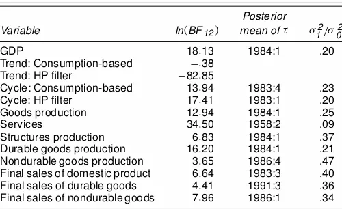
Table 1. Bayesian Evidence of a Volatility Reduction in Aggregate and Disaggregate Real GDP
Posterior
Variable ln.BF12/ mean of¿ ¾2
1=¾02
GDP 18:13 1984:1 .20
Trend: Consumption-based ¡:38
Trend: HP lter ¡82:85
Cycle: Consumption-based 13:94 1983:4 .23
Cycle: HP lter 17:41 1983:1 .20
Goods production 12:94 1984:1 .25
Services 34:50 1958:2 .09
Structures production 6:83 1984:1 .37
Durable goods production 16:20 1984:1 .21
Nondurable goods production 3:65 1986:4 .47
Final sales of domestic product 6:64 1983:3 .40
Final sales of durable goods 4:41 1991:3 .36
Final sales of nondurable goods 7:96 1986:1 .34
structural break, model 2, withkD6 the largest lag length con-sidered. The AIC chose two lags for all series except consump-tion of nondurable goods and services, for which it chose one lag. All inferences are based on 10,000 Gibbs simulations, af-ter the initial 2,000 simulations were discarded to mitigate the effects of initial conditions.
Table 1 summarizes the results of the Bayesian estimation and model comparisons for all of the aggregate and disaggre-gate real GDP series considered. The second column presents the results of the Bayesian model comparison, summarized by the log of the Bayes factor in favor of a structural break, ln.BF12/. The third column shows the mean of the posterior distribution of the break date,¿. The fourth column presents the ratio of posterior means of the variance ofetbefore and after
the structural break,¾12=¾02. Finally, Figures 1–13 plot the esti-mated probability of a structural break at each point in the sam-ple, Pr.DtD1jeYT/, and the posterior distribution of the break
date for each series considered.
3.1 Aggregate Real GDP, Trend, and Cycle
The rst row of Table 1 contains results for the growth rate of aggregate real GDP. The posterior mean of¾12is 20% of¾02,
(a) (b)
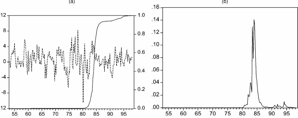
Figure 1. Growth Rate of GDP: (a) Probability of Structural Break; and (b) Posterior Distribution of Break Date.
(a) (b)
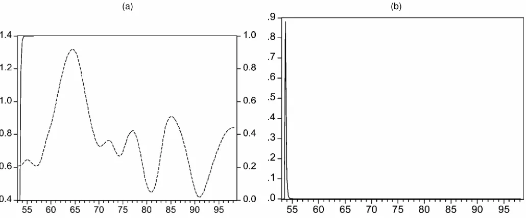
Figure 2. Growth Rate of Consumption of Nondurable Goods and Services: (a) Probability of Structural Break; and (b) Posterior Distribution of Break Date.
consistent with a sizable reduction in conditional volatility. The log of the Bayes factor is 18.1, decisive evidence against the model with no volatility reduction. The posterior mean of the unknown break date is 1984:1, the same date reported by Kim and Nelson (1999) and MPQ. Figure 1(b) shows that the poste-rior distribution of the unknown break date is tightly clustered around its mean.
We next turn to the question of whether both the trend and the cyclical component of real GDP have shared in this ag-gregate volatility reduction. It seems reasonable that at least a portion of the volatility reduction is due to a stabilization of cyclical volatility. Many plausible explanations for the volatil-ity reduction (e.g., improved monetary policy and better inven-tory management) would mute cyclical uctuations. However, some explanations (e.g., a lessening of oil price shocks) might also affect the variability of trend growth rates. Thus investi-gating a stabilization in the trend and cyclical components may
help shed light on the viability of competing explanations for the aggregate volatility reduction.
There are, of course, numerous ways of decomposing real GDP into a trend and cyclical component. Unfortunately, the choice of decomposition can have nontrivial implications for implied business cycle facts (see, e.g., Canova 1998). This seems particularly relevant for investigating a structural break in volatility, because assumptions made to identify the trend may affect how much of a volatility reduction in the aggregate series is reected in the ltered trend or cycle. To abstract from this problem, in this article we consider a theory-based mea-sure of trend, dened as the logarithm of personal consump-tion of nondurables and services (LCNDS). Such a deniconsump-tion of trend is both theoretically and empirically plausible. Neo-classical growth theory (see, e.g., King, Plosser, and Rebelo 1988) suggests that log real GDP and LCNDS share a common stochastic trend driven by technological change. This analy-sis suggests that log real GDP and LCNDS are cointegrated
(a) (b)
Figure 3. Growth Rate of HP Trend: (a) Probability of Structural Break; and (b) Posterior Distribution of Break Date.
(a) (b)
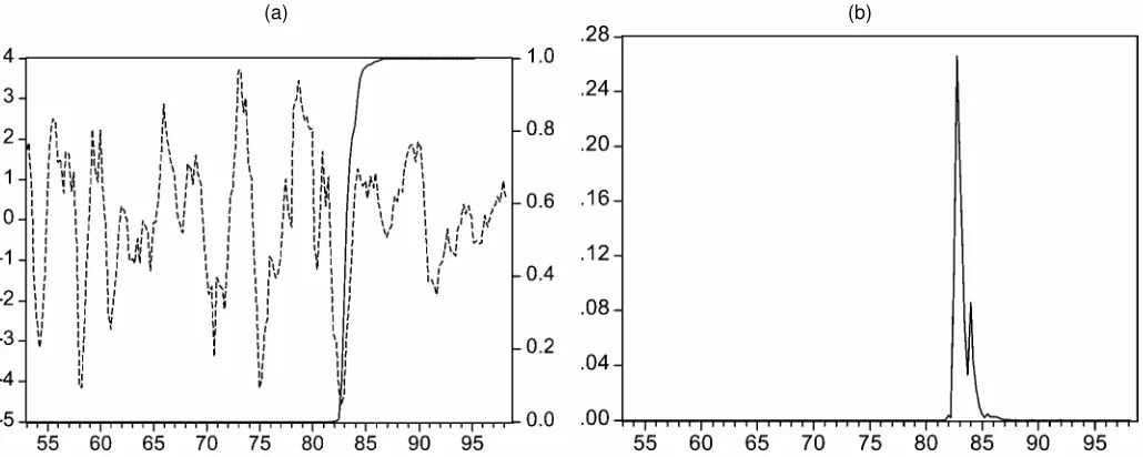
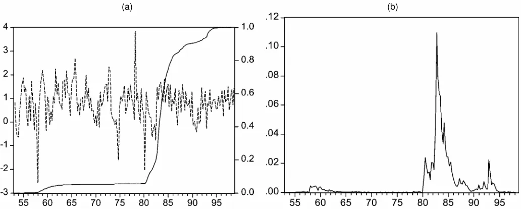
Figure 4. Consumption-Based Cycle: (a) Probability of Structural Break; and (b) Posterior Distribution of Break Date.
with cointegrating vector.1;¡1/. Recent investigations of the cointegration properties of these series conrm this result (see, e.g., King, Plosser, Stock, and Watson 1991; Bai, Lumsdaine, and Stock 1998). If one also assumes a simple version of the permanent income hypothesis, which suggests that LCNDS is a random walk, then LCNDS is the common stochastic trend shared by log real GDP and LCNDS. Although it is now well known that LCNDS is not a random walk, in the sense that one can nd statistically signicant predictors of future changes in LCNDS, Fama (1992) and Cochrane (1994) have argued that these deviations are so small as to be economically insignif-icant. Based on our measure of trend, we dene the cyclical component of log real GDP as the residuals from a regression of log real GDP on a constant and LCNDS. Given its popularity, we also show results for a measure of trend and cycle obtained from the Hodrick–Prescott (H–P) lter with smoothing parame-ter set equal to 1,600.
The second row of Table 1 shows that there is no evidence in favor of a break in the volatility of the growth rate of LCNDS
and thus in the growth rate of our theory-based measure of the trend of log real GDP. The log of the Bayes factor is¡:4, pro-viding slight evidence in favor of model 2, the model with no change in variance. The third column of Table 1 shows that the evidence for a break in the growth rate of the H–P measure of trend is even weaker, with model 2 strongly preferred over model 1. This suggests that the volatility reduction observed in aggregate real GDP is focused in its cyclical component. In-deed, the log of the Bayes factor for the level of the cyclical component derived from the theory-based measure of trend, re-ported in the fourth row of Table 1, is 13.9, providing decisive evidence against model 1. The posterior mean of¾12 is 23% of¾02, close to the percentage for aggregate GDP. The posterior mean of the unknown break date is 1983:4 with [from Fig. 3(b)] the posterior distribution of the break point clustered tightly around this mean. Even stronger results are obtained for the cyclical component based on the H–P lter, shown in the fth row of Table 1. Here the posterior mean of¾12is 20% of¾02and
(a) (b)
Figure 5. HP Cycle: (a) Probability of Structural Break; and (b) Posterior Distribution of Break Date.
(a) (b)
Figure 6. Growth Rate of Goods Production: (a) Probability of Structural Break; and (b) Posterior Distribution of Break Date.
the log Bayes factor is 17.4. These results, which suggest that only the cyclical component of real GDP has undergone a large volatility reduction, makes explanations for the aggregate stabi-lization based on a reduction of shocks to the trend component less compelling.
3.2 How Broad Is the Volatility Reduction? Evidence From Disaggregate Data
In this section we attempt to evaluate the pervasiveness of the volatility reduction observed in aggregate real GDP across sec-tors of the economy. To this end, we apply the Bayesian testing methodology to the set of disaggregated real GDP data inves-tigated by MPQ. This dataset comprises the broad production sectors of real GDP: goods production,services production,and structures production. We investigate goods production further by separating durable goods and nondurable goods production. Finally, we investigate the evidence for a volatility reduction in measures of nal sales in the goods sector. MPQ found a
volatility reduction only in the productionof durable goods, and determined that the volatility reduction was not visible in mea-sures of nal sales. Thus we are particularly interested in the evidence for a volatility reduction outside of the durable goods sector and in measures of nal sales.
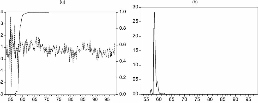
Rows 6–8 of Table 1 contain the results for the production of goods, services, and structures. Consistent with MPQ, we nd strong evidence of a volatility reduction in the goods sec-tor. The log of the Bayes factor for goods production is 12.9, providing decisive evidence against the model with no change in volatility. The volatility reduction is quite large, with the posterior mean of¾12 25% of ¾02. The posterior mean of the break date is 1984:1, close to the date estimated by MPQ using classical techniques. Also consistent with MPQ, we nd little evidence of a volatility reduction in services production that oc-curs around the time of the break in aggregate real GDP. From row 7 of Table 1, the log Bayes factor for services production is 34.5, extremely strong evidence in favor of a volatility reduc-tion. However, the estimated mean of the break date is 1958:2,
(a) (b)
Figure 7. Growth Rate of Services: (a) Probability of Structural Break; and (b) Posterior Distribution of Break Date.
(a) (b)
Figure 8. Growth Rate of Structures Production: (a) Probability of Structural Break; and (b) Posterior Distribution of Break Date.
not in the early 1980s. Figure 7(b) conrms this, showing no mass in the posterior distribution of the break date in the 1980s. However, because the model used here allows for only a single structural break, there may be evidence of a second structural break in the early 1980s that is not captured. To investigate this possibility, we re-estimated the model for services production using data beginning in 1959. The log Bayes factor fell to 3.4, still strong evidence for a structural break. However, the esti-mated break date was again well before the early 1980s, with the mean of the posterior distribution in the second quarter of 1966.
We turn now to structures production, where we obtain the rst discrepancy with the results obtained by MPQ. Again, using classical tests, MPQ were unable to reject the null hy-pothesis of no structural break in the conditional volatility of structures production. However, the Bayesian tests nd deci-sive evidence of a volatility reduction. From row 8 of Table 1, the log Bayes factor is 6.8, with the posterior mean of the break date equal to 1984:1, the same quarter as for aggregate GDP.
Figure 8(b) shows that the posterior distribution of the break date is clustered tightly around the posterior mean. The volatil-ity reduction in structures is quantitatively large as well; the posterior mean of¾12 is 37% of¾02. Thus the evidence from the Bayesian model comparison suggests that the volatility re-duction observed in real GDP not only is reected in the goods sector, as suggested by MPQ, but also is found in the production of structures.
Following MPQ, we next delve deeper into an evaluation of the goods sector by separately evaluating the evidence for a volatility reduction in the nondurable and durable goods sec-tors. Row 9 of Table 1 contains the results for durable goods. The log Bayes factor is 16.2, decisive evidence in favor of structural change. The posterior mean of the unknown break date is the same as for aggregate GDP, 1984:1. From row 10, the log Bayes factor for nondurable goods production is 3.7, smaller than for durable goods but still strong evidence against the model with no structural break. The volatility reduction in
(a) (b)
Figure 9. Growth Rate of Durable Goods Production: (a) Probability of Structural Break; and (b) Posterior Distribution of Break Date.
(a) (b)
Figure 10. Growth Rate of Nondurable Goods Production: (a) Probability of Structural Break; and (b) Posterior Distribution of Break Date.
nondurablegoods is quantitativelylarge, with¾1247% of¾02, al-though smaller than that found for durable goods. The posterior mean of the break date is also somewhat later than for durable goods, falling in 1986:4. Finally, from Figures 9(b) and 10(b), the posterior distribution of the break date for nondurablegoods production is more diffuse than those for durable goods produc-tion.
We now turn to an investigation of measures of nal sales. Again, a striking result found by MPQ is that classical tests do not reject the null hypothesis of no volatility reduction for either aggregate measures of nal sales or nal sales of durable goods. This result is strongly suggestive of a primary role for the be-havior of inventories in explaining the aggregate volatility re-duction. MPQ also argued that the failure of nal sales to show any evidence of a volatility reduction casts doubt on explana-tions for the aggregate volatility reduction based on monetary policy. To investigate the possibility of a volatility reduction in
nal sales, we investigate three series. The rst series is an ag-gregate measure of nal sales—nal sales of domestic product. We then turn to measures of nal sales in the goods sector. In particular, we investigate nal sales of nondurable goods and nal sales of durable goods.
From row 11 of Table 1, the log of the Bayes factor for -nal sales of domestic product is 6.6, decisive evidence against the model with no volatility reduction. The volatility reduction in nal sales is quantitatively large, with the posterior mean of
¾1240% of¾02. The posterior mean of the break date is 1983:3, consistent with that observed for aggregate real GDP. From Fig-ure 11(b), the posterior distribution is clustered fairly tightly around this mean, although less so than for aggregate real GDP. That we nd evidence for a volatility reduction in aggregate -nal sales is perhaps not surprising given that we have already shown that the Bayesian model comparison nds evidence of a structural break in structures production, a component of ag-gregate nal sales. Thus we are perhaps more interested in the
(a) (b)
Figure 11. Growth Rate of Final Sales of Domestic Product: (a) Probability of Structural Break; and (b) Posterior Distribution of Break Date.
(a) (b)
Figure 12. Growth Rate of Durable Goods Final Sales: (a) Probability of Structural Break; and (b) Posterior Distribution of Break Date.
results with regard to nal sales in the goods sector, the only sector for which the distinction between sales and production is meaningful. We now turn to these results.
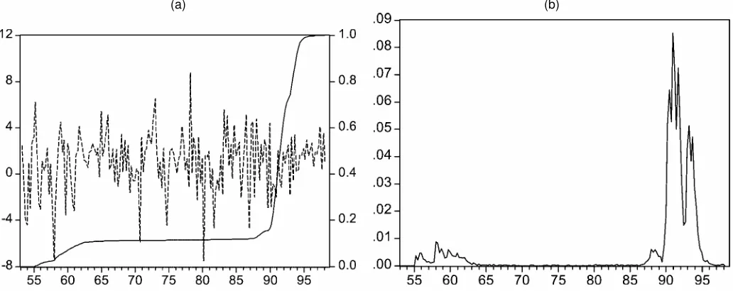
From row 12 of Table 1, the log of the Bayes factor for -nal sales of durable goods is 4.4, strong evidence against the model with no structural break. However, the log Bayes factor is weaker than when inventories are included, suggesting that inventory behavior may be an important part of the volatility reduction in durable goods production in the early 1980s. Also, the posterior mean of the break date for nal sales of durable goods is in 1991:3. This break is 7 years later than that recorded for aggregate GDP and durable goods production. Thus it ap-pears that the MPQ nding of no volatility reduction in nal sales of durable goods is not conrmed by the Bayesian tech-niques used here. However, there does appear to be signicant timing differences in volatility reduction in the production and nal sales of durable goods.
From row 13 of Table 1, we see that there is much ev-idence of a volatility reduction in nal sales of nondurable goods. The log Bayes factor is 8.0, decisive evidence against the model with no structural break. Interestingly, this is much stronger evidence than that obtained for the production of non-durable goods. Also, the volatility reduction for nal sales of nondurable goods appears to be quantitatively more important than that for production of nondurables, with¾1234% of¾02for nondurable nal sales and 47% of¾02for nondurable produc-tion. The posterior mean of the break date is in 1986:1, close to the break date for nondurable goods production. However, as seen in Figure 13(b), the posterior distribution of the break date is much more tightly clustered around this mean than that obtained for nondurable goods production. Thus the results for nal sales of nondurable goods suggests the opposite conclu-sion than was obtained for durable goods: The evidence in favor of a break in volatility in the nondurable goods sector is more compelling when only nal sales are considered. This could be
(a) (b)
Figure 13. Growth Rate of Nondurable Goods Final Sales: (a) Probability of Structural Break; and (b) Posterior Distribution of Break Date.
used as evidence against an inventory management explanation for the volatility reduction in this sector.
In summary, the evidence presented here demonstrates that the results of MPQ are not robust to a Bayesian model compar-ison strategy. Specically, the volatility reduction appears to be pervasive across many of the production components of aggre-gate real GDP and is also present in measures of nal sales in addition to production. This evidence provides less ammunition to invalidate any potential explanation for the aggregate volatil-ity reduction than that obtained by MPQ. Indeed, the evidence seems consistent with a broad range of explanations, includ-ing improved inventory management and improved monetary policy, and thus is not very helpful in narrowing the eld of potential explanations.
One could still argue that our nding of reduced volatility of durable goods production in 1984, with no reduction in durable nal sales volatility until 1991, makes improved inventory man-agement the leading candidate explanation for the volatility re-duction within the durable goods sector. However, even this may not be a useful conclusion to draw from the stylized facts. The results presented here suggest a difference in timing only, not the absence of a volatility reduction in the nal sales of durables goods as in MPQ. Such a timing difference could be explained by many factors, including idiosyncratic shocks to nal sales over the second half of the 1980s. Another explana-tion is that the hypothesis of a single, sharp break date is mis-specied, and in fact volatility reduction has been an ongoing process. Stock and Watson (2002) and Blanchard and Simon (2001) have presented evidence that is not inconsistent with this hypothesis. If this is the true nature of the volatility reduc-tion, then the discrepancy in the estimated (sharp) break date for durable goods production and nal sales of durable goods becomes less interesting.
3.3 Robustness to Alternative Prior Specications
We obtained the results presented in Section 3.2 using the prior parameter distributions listed as “prior 1A” in Section 2. We also estimated the model with priors 1B and 1C and ob-tained results very similar to those given in Table 1. In this sec-tion we further evaluate the sensitivity of the results to prior specication by investigating alternative priors on the Markov transition probability,q. This is a key parameter of the model, because it controls the placement of the unknown break date. Thus the econometrician can specify beliefs regarding the tim-ing of the structural break by modifytim-ing the prior distribution for q. Classical tests, such as those of Andrews (1993) and Andrews and Ploberger (1994), assume no prior knowledge of the break date. Thus we are interested in the extent to which the differences between the results that we nd here and those obtained by MPQ can be explained by the prior distributions placed onq.
We investigate this by re-evaluating one of the primary se-ries considered earlier for which we draw differing conclusions from MPQ—structures production. Using classical tests, MPQ were unable to reject the null hypothesis of no structural break in the volatility of structures production. Here we found a log Bayes factor of model 1 versus model 2 of 6.8, strong evi-dence in favor of a structural break. We obtained this factor
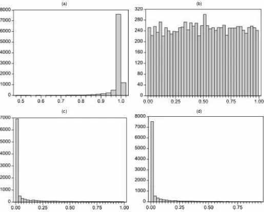
using the prior onqlisted in prior 1A,q»beta.8; :1/, the his-togram of which, based on 10,000 simulated draws from the distribution, is plotted in Figure 14(a). This distribution has meanE.q/¼:988 and standard deviation .037. How restric-tive is this prior onq for the placement of the break date¿? From the 10,000 draws ofq plotted in Figure 14(a), roughly 80% corresponded toE.¿ /D1=.1¡q/ >90 quarters, which is the midpoint of the sample size considered in this article. Cor-respondingly, roughly 20% of the draws from the distribution forqyielded expected break dates less than 90 quarters into the sample.
Table 2 considers the robustness of the result for structures production to alternative prior specications onq, keeping the prior distributions for the other parameters of the model the same as in prior 1A. Figure 14(b) holds the histogram for the rst alternative prior that we consider,q»beta.1;1/. This prior is relatively at, with mean equal to .5 and roughly equal prob-ability placed on all values ofq. However, this yields a some-what more restrictive prior distribution for the placement of the break date,¿, than that used in prior 1A. From the 10,000 draws ofq plotted in Figure 14(b), only 1% corresponded to E.¿ /D1=.1¡q/ >90 quarters. Furthermore, 98% of the draws ofqyielded expected break dates in the rst 50 quarters of the sample. From the second row of Table 2, the log Bayes fac-tor for this prior specication is 3.7, less than that obtained us-ing prior 1A but still strong evidence in favor of a structural break. We next investigate a prior that places the mean value ofq at a very low value, thus placing most probability mass on a break date early in the sample. We specify this prior as q»beta.:1;1/, the histogram of which is contained in Fig-ure 14(c). This prior could be considered quite unreasonable. From the 10,000 draws ofqplotted in Figure 14(c), less than .1% corresponded to E.¿ /D1=.1¡q/ >90 quarters. More-over, more than 99% of the draws ofqyielded expected break dates in the rst 12 quarters of the sample. However, despite this unreasonable prior, the log Bayes factor, shown in the third row of Table 2, is still above 3, strong evidence in favor of a structural break. To erase the evidence in favor of a structural break, one must move to the prior in the nal row of Table 2, q»beta.:1;2/. This prior distribution, graphed in Figure 14(d), places almost all probability mass on a break very early in the sample. Of the 10,000 draws ofqplotted in Figure 14(d), none corresponded to E.¿ /D1=.1¡q/ >50 quarters. Under this prior, the model with no structural break is preferred slightly over the model with a structural break.
Thus it appears that the evidence for a structural break in structures production is robust to a wide variety of prior distri-butions. This suggests that the sample evidence for a structural break is quite strong, making the choice of prior distribution on the break date of limited importance for conclusions based on Bayes factors.
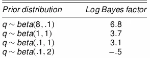
Table 2. Evidence of Structural Break for Alternative Priors on q:
Structures Production
Prior distribution Log Bayes factor
q»beta.8; :1/ 6:8
q»beta.1;1/ 3:7
q»beta.:1;1/ 3:1 q»beta.:1;2/ ¡:5
(a) (b)
(c) (d)
Figure 14. Histogram for (a) 10,000 Draws From q»beta(8; :1), (b) 10,000 Draws From q»beta(1;1), (c) 10,000 Draws From q»beta(:1;1), and (d) 10,000 Draws From q»beta(:1;2).
3.4 Structural Change in Ination Dynamics
In this section we evaluate whether the reduction in the volatility of real GDP is also present in the dynamics of in-ation. Unlike the case of real GDP, changes in conditional mean and persistence also appear to be important for ination. Thus, to investigate structural change in the dynamics of ina-tion, we use the following expanded version of the model in Section 2:
ytD¹D¤t C½D¤tyt¡1C
p¡1
X
jD1
¯j;D¤t1yt¡jCet;
et»N
¡
0; ¾D2
t
¢
;
(3)
where yt is the level of the ination rate. The specication
of the error term and its variance is the same as that in Section 2. However, we also allow for a structural break in the persistence parameter and conditional mean. For exam-ple, whereas ¾D2
t captures a shift in conditional volatility, the parameter ½D¤
t, which is the sum of the autoregressive coef-cients in the Dickey–Fuller style autoregression, captures a
one-time shift in the persistence. We allow for the possibil-ity that a shift in the persistence parameter and conditional mean can occur at a different time than the shift in condi-tional variance. Thus we assume thatD¤t is independent ofDt
and that it is governed by the following transitional dynam-ics:
D¤t D
»
0 1·t·¿¤
1 ¿¤<t<T¡1, Pr.D¤tC1D0jD¤t D0/Dq¤;
Pr.D¤tC1D1jD¤t D1/D1:
(4)
For ination, we consider a shorter sample period than for the real variables, beginning in the rst quarter of 1960. Pre-liminary analysis suggested that including data from the 1950s yielded very unstable results that were generally indicative of a structural break in the dynamics of the series in the late 1950s. That the 1950s might represent a separate regime in the be-havior of ination is perhaps not surprising. Romer and Romer (2002) argued that monetary policy in the 1950s had more in
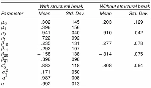
Table 3. Posterior Moments: CPI Ination
With structural break Without structural break
Parameter Mean Std. Dev. Mean Std. Dev.
¹0 :302 .145 :203 .129
¹1 :396 .156
½0 :941 .040 :910 .042
½1 :722 .092
¯10 ¡:235 .131 ¡:277 .078 ¯11 ¡:292 .107
¯20 ¡:158 .138 ¡:314 .075 ¯21 ¡:398 .098
¾02 :883 .118 :808 .094
¾12 :171 .050
q¤ :987 .008
q :992 .013
common with that in the 1980s and 1990s than that in the 1960s and 1970s. Because here we are interested in a structural break that corresponds to the break found in real variables in the early 1980s, we restrict our attention to the post-1960s sample. This is a common sample choice in studies investigating structural change in U.S. nominal variables (see, e.g., Watson 1999; Stock and Watson 2002).
Table 3 contains the mean and standard deviation of the pos-terior distributions for the parameters of the model in (3) and (4) applied to the consumer price index ination rate. The log of the Bayes factor comparing this model with one with no struc-tural breaks is 7.8, decisive evidence against the model with no structural change. The structural change appears to be coming from two places, a reduction in persistence and a reduction in conditional variance. The posterior mean of the persistence pa-rameter falls from½0D:94 to½1D:72. The posterior mean of
the conditional volatility falls from¾02D:88 to¾12D:17. The conditionalmean, given by¹0and¹1, is essentially unchanged
over the sample. Figure 15(b) shows the posterior distributions of the two break dates. The break date for the change in per-sistence, ¿¤, and the change in volatility,¿, both have
poste-rior distributions clustered tightly around their posteposte-rior means, 1979:2 and 1991:2. Given that the reduction in persistence im-plies a reduction in unconditional volatility, these results sug-gest two reductions in volatility, one reduction at the beginning of the 1980s and another at the beginning of the 1990s.
4. WHAT EXPLAINS THE DISCREPANCY BETWEEN THE CLASSICAL AND BAYESIAN RESULTS?
The results of MPQ and this article demonstrate that for sev-eral of the disaggregate real GDP series, classical tests fail to reject the null hypothesis of no volatility reduction, whereas a Bayesian model comparison strongly favors a volatility reduc-tion. One simple explanation for this discrepancy is that clas-sical hypothesis tests and Bayesian model comparisons are in-herently very different concepts. Whereas classical hypothesis tests evaluate the likelihood of observing the data assuming that the null hypotheses is true, a Bayesian model comparison eval-uates which of the null or alternative hypotheses is more likely. Given this difference in philosophy, the approach preferred by a researcher will likely depend on that researcher’s preferences for classical versus Bayesian techniques.
This explanation is somewhat unsatisfying, because it sug-gests that “frequentist” researchers will prefer the results of MPQ, whereas “Bayesian” researchers will nd the results pre-sented in this article more convincing. Thus in the remainder of this section, we report on a series of Monte Carlo experi-ments performed to explore the discrepancy between the two procedures from a purely classical perspective. Based on the results of these experiments, we argue that for this application, the conclusionsfrom the Bayesian model comparison should be preferred, even when viewed from the viewpoint of a classical econometrician.
We rst consider the case in which a volatility reduction has occurred in the series for which the classical and Bayesian
(a) (b)
Figure 15. CPI Ination Rate: (a) Probability of Structural Break; and (b) Posterior Distribution of Break Date.
methodologies provide conicting results. In this case, the Bayesian model comparison correctly identies the true model, whereas the classical hypothesis test fails to reject the false null hypothesis, a type II error. Given that the alternative hypothesis is true, how likely would it be to observe this type II error? To answer this question, we perform a Monte Carlo experiment to calculate the power of a classical test used by MPQ against two relevant alternative hypotheses. In the rst of these hypotheses, (DGP1), data are generated from an autoregression in which there is an abrupt change in the residual variance. Formally,
ytD¹CÁ1yt¡1CÁ2yt¡2Cet;
In the second hypothesis, (DGP2), data are generated from an autoregression in which there is a gradual change in the residual variance,
DGP2 is motivated by the posterior distributions of¿ for the disaggregate real GDP data series. As is apparent from Fig-ures 6–13, the posterior distribution of ¿ is fairly diffuse in several cases, a result suggestive of gradual, rather than sharp, structural breaks. Notably, this tends to be the case for those series for which the results of MPQ differ from the Bayesian model comparison: structures production, nondurable goods production, and all of the nal sales series.
We base the calibration of DGP1 and DGP2 on a series for which the classical and Bayesian methodologies are sharply at odds: nal sales of domestic product. For this series, the log Bayes factor is 6.64, decisive evidence against the null of no structural change. However, MPQ were unable to reject the null hypothesis of no structural change in this series using classical tests. We replicate this result here using the Quandt (1960) sup-Waldtest statistic, the critical values of which were derived by Andrews (1993). Following MPQ, we perform this test based on the following equation for the residuals of (5):
jetj D®0.1¡Dt/C®1DtC!t;
then estimate (7) by least squares and the Wald statistic for the test of the null hypothesis that ®0 D®1 calculated for
each potential value of¿. Again following MPQ, we use 15% trimming—the break date is not allowed to occur in the rst or
last 15% of the sample. The largest test statistic obtained is the sup-Waldstatistic, whereas the value of¿ that yields the sup-Waldstatistic is the least squares estimate of the break date,¿O. Consistent with MPQ, thesup-Waldtest statistic for nal sales of domestic product is 7.05, below the 5% critical value of 8.85. To calibrate DGP1, we set the parameter¿ D O¿ for nal sales of domestic product. The parameters¹,Á1, andÁ2are then set
equal to their ordinary least squares estimates from (5), where the estimation is performed conditional on¿ D O¿. Finally,¾02
and¾12are set equal to
estimation of model 1, dened in Section 2.1, for nal sales of domestic product. This probability is displayed in Figure 11(a). We set the other parameters equal to the means of the respec-tive posterior distributions from estimation of model 1 for nal sales of domestic product. We generate 10,000 sets of data from DGP1 and DGP2, each set with a length equal to the sample size of our series for nal sales of domestic product. For each dataset generated, we perform a 5%sup-Waldtest and record whether the null hypothesis is rejected.
For DGP1, thesup-Waldstatistic rejects the null hypothesis 75% of the time, suggesting that the power of this test against DGP1 is only fair. Under DGP2, arguably the more relevant data-generating process for the disputed series, the power of thesup-Waldtest falls considerably, with the test rejecting only 43% of the time. Thus these results suggest that if the alternative hypothesis were true, then it would not be unlikely for the sup-Waldtest to fail to reject the null hypothesis. This provides a possible reconciliation of the discrepancy between the classical and Bayesian results.
We next turn to the case in which the null hypothesis is true. In this case, the classical tests used by MPQ correctly fail to reject the null hypothesis, whereas the Bayesian model com-parison, calibrated to Jeffreys’s scale, incorrectly prefers the al-ternative hypothesis. From a classical perspective, the Bayesian model comparison commits a type I error. Thus, another possi-ble reconciliationof the conicting results given by the classical and Bayesian methodologies is that the Bayesian model com-parison tends to commit a larger number of type I errors than the classical test. The question then is if the Bayes factor as in-terpreted in this article were treated as a classical test statistic, what would its size be?
To investigate this, we perform a Monte Carlo experiment where data are generated under the null hypothesis of no struc-tural change. Specically, we generate data from model 2 de-scribed in Section 2. We calibrated the parameters to the means of the posterior distributions for the parameters of model 2 t to nal sales of domestic product. For each Monte Carlo simu-lation, we computed the log Bayes factor, using the same priors as dened in Section 2. Due to the lengthy computation time required for each simulation, we reduced the number of Monte Carlo simulations to 1,000.
In this experiment, 5% of the log Bayes factors exceeded 3.4. Thus, if one were to treat the log Bayes factor as a clas-sical test statistic, then the 5% critical value would be 3.4. In
the results reported in Table 1, the log Bayes factor exceeds this value in all cases except the two measures of trend GDP. This suggests that the discrepancy in the results of MPQ and the Bayesian model comparison are not likely to be explained by the Bayesian model comparison having an excessive size when viewed as a classical test. Indeed, given that the values of the Bayes factors in Table 1 are often far above the 5% critical value of 3.4, this reconciliation seems very unlikely.
In summary, these Monte Carlo experiments suggest that when viewed from a classical perspective, it would not be un-usual for classical tests to fail to reject the null hypothesis when the alternative was the correct model. However, it would be highly unlikely to observe values for the log Bayes factor as large as those observed in Table 1 if the null hypothesis of no structural change were true.
5. CONCLUSION
In this article we used Bayesian tests for a structural break in variance to document some stylized facts regarding the volatil-ity reduction in real GDP observed since the early 1980s. First, we found a reduction in the volatility of aggregate real GDP that is shared by its cyclical component but not by its trend component. Next, we investigated the pervasiveness of this ag-gregate volatility reduction across broad production sectors of real GDP. Evidence from the existing literature based on clas-sical testing procedures has shown that the aggregate volatility reduction has a narrow source—the durable goods sector—and that measures of nal sales fail to show any volatility reduc-tion. This evidence has been used to cast doubt on explanations for the volatility reduction based on improved monetary policy. In contrast, we have found that the volatility reduction in ag-gregate output is visible in more sectors of output than simply durable goods production. Specically, we found evidence of a volatility reduction in the production of structures and non-durable goods. We also found evidence of a reduced volatility of aggregate measures of nal sales similar to that in aggregate output. Finally, we found evidence of reduced volatility in nal sales of both durable goods and nondurable goods. Based on these results, we argue that the evidence that one obtains from investigating the pattern of volatility reductions across broad production sectors of real GDP is not sufciently sharp to cast doubt on any potential explanations for the volatility reduction. We also document that, alongside the reduction in real GDP volatility, the persistence and conditional volatility of ination have also fallen.
ACKNOWLEDGMENTS
Chang-Jin Kim and Charles R. Nelson acknowledge support from National Science Foundation grant SES-9818789, Kim acknowledges support from a Korea University special grant, and Jeremy Piger acknowledges support from the Grover and Creta Ensley Fellowship in Economic Policy at the University of Washington. The authors thank without implicating Mark Gertler, Andrew Levin, James Morley, the editor, associate edi-tor, an anonymousreferee, and seminar participants at the Johns
Hopkins University, University of Washington, Federal Reserve Board, and the 2001 AEA annual meeting for helpful com-ments. The views expressed in this article do not necessarily represent ofcial positions of the Federal Reserve Bank of St. Louis or the Federal Reserve System.
[Received August 2000. Revised March 2003.]
REFERENCES
Ahmed, S., Levin, A., and Wilson, B. A. (2002), “Recent U.S. Macroeconomic Stability: Good Policy, Good Practices, or Good Luck?” International Fi-nance Discussion Paper no. 730, Board of Governors of the Federal Reserve System.
Andrews, D. W. K. (1993), “Tests for Parameter Instability and Structural Change With Unknown Change Point,”Econometrica, 61, 821–856. Andrews, D. W. K., and Ploberger, W. (1994), “Optimal Tests When a Nuisance
Parameter Is Present Only Under the Alternative,”Journal of Econometrics, 70, 9–38.
Bai, J., Lumsdaine, R. L., and Stock, J. H. (1998), “Testing for and Dating Common Breaks in Multivariate Time Series,”Review of Economic Studies, 65, 395–432.
Blanchard, O., and Simon, J. (2001), “The Long and Large Decline in U.S. Output Volatility,”Brookings Papers on Economic Activity, 1, 135–174. Canova, F. (1998), “Detrending and Business Cycle Facts,”Journal of
Mone-tary Economics, 41, 475–512.
Chauvet, M., and Potter, S. (2001), “Recent Changes in U.S. Business Cycle,”
The Manchester School, 69, 481–508.
Chib, S. (1995), “Marginal Likelihood From the Gibbs Output,”Journal of the American Statistical Association, 90, 1313–1321.
(1998), “Estimation and Comparison of Multiple Change-Point Mod-els,”Journal of Econometrics, 86, 221–241.
Cochrane, J. H. (1994), “Permanent and Transitory Components of GNP and Stock Prices,”Quarterly Journal of Economics, 109, 241–263.
Fama, E. F. (1992), “Transitory Variation in Investment and Output,”Journal of Monetary Economics, 30, 467–480.
Jeffreys, H. (1961),Theory of Probability(3rd ed.), Oxford, U.K.: Clarendon Press.
Kahn, J., McConnell, M. M., and Perez-Quiros, G. P. (2000), “The Reduced Volatility of the U.S. Economy: Policy or Progress?” mimeo, Federal Reserve Bank of New York.
Kass, R. E., and Raftery, A. E. (1995), “Bayes Factors,”Journal of the American Statistical Association, 90, 773–795.
Kim, C.-J., and Nelson, C. R. (1999), “Has the U.S. Economy Become More Stable? A Bayesian Approach Based on a Markov-Switching Model of the Business Cycle,”Review of Economics and Statistics, 81, 608–616. King, R. G., Plosser, C. I., and Rebelo, S. T. (1988), “Production, Growth and
Business Cycles II: New Directions,”Journal of Monetary Economics, 21, 309–341.
King, R. G., Plosser, C. I., Stock, J. H., and Watson, M. W. (1991), “Sto-chastic Trends and Economic Fluctuations,”American Economic Review, 81, 819–840.
Koop, G., and Potter, S. M. (1999), “Bayes Factors and Nonlinearity: Evidence From Economic Time Series,”Journal of Econometrics, 88, 251–281. McConnell, M. M., and Perez-Quiros, G. P. (2000), “Output Fluctuations in
the United States: What Has Changed Since the Early 1980s?”American Economic Review, 90, 1464–1476.
Niemira, M. P., and Klein, P. A. (1994),Forecasting Financial and Economic Cycles, New York: John Wiley & Sons, Inc.
Quandt, R. (1960), “Tests of the Hypothesis That a Linear Regression Obeys Two Separate Regimes,”Journal of the American Statistical Association, 55, 324–330.
Romer, C. D., and Romer, D. H. (2002), “A Rehabilitation of Monetary Pol-icy in the 1950’s,”American Economic Review Papers and Proceedings, 92, 121–127.
Stock, J. H., and Watson, M. W. (2002), “Has the Business Cycle Changed and Why?”NBER Macroeconomics Annual, 17, 159–218.
Warnock, M. V., and Warnock, F. E. (2000), “The Declining Volatility of U.S. Employment: Was Arthur Burns Right?” International Finance Discussion Paper no. 677, Board of Governors of Federal Reserve System.
Watson, M. W. (1999), “Explaining the Increased Variability of Long-Term In-terest Rates,”Federal Reserve Bank of Richmond Economic Quarterly, Fall 1999.