Full Terms & Conditions of access and use can be found at
http://www.tandfonline.com/action/journalInformation?journalCode=ubes20
Download by: [Universitas Maritim Raja Ali Haji] Date: 12 January 2016, At: 22:50
Journal of Business & Economic Statistics
ISSN: 0735-0015 (Print) 1537-2707 (Online) Journal homepage: http://www.tandfonline.com/loi/ubes20
Health Risk and Portfolio Choice
Ryan D Edwards
To cite this article: Ryan D Edwards (2008) Health Risk and Portfolio Choice, Journal of
Business & Economic Statistics, 26:4, 472-485, DOI: 10.1198/073500107000000287
To link to this article: http://dx.doi.org/10.1198/073500107000000287
Published online: 01 Jan 2012.
Submit your article to this journal
Article views: 306
Health Risk and Portfolio Choice
Ryan D. E
DWARDSDepartment of Economics, Queens College, CUNY, Flushing, NY 11367 (redwards@qc.cuny.edu)
This article investigates the role of self-perceived risky health in explaining continued reductions in finan-cial risk taking after retirement. If future adverse health shocks threaten to increase the marginal utility of consumption, either by absorbing wealth or by changing the utility function, then health risk should prompt individuals to lower their exposure to financial risk. I examine individual-level data from the Study of Assets and Health Dynamics Among the Oldest Old (AHEAD), which reveal that risky health prompts safer investment. Elderly singles respond the most to health risk, consistent with a negative cross partial deriving from health shocks that impede home production. Spouses and planned bequests provide some degree of hedging. Risky health may explain 20% of the age-related decline in financial risk taking after retirement.
KEY WORDS: Background risk; Cross partial derivative; Precautionary saving; State-dependent utility.
1. INTRODUCTION
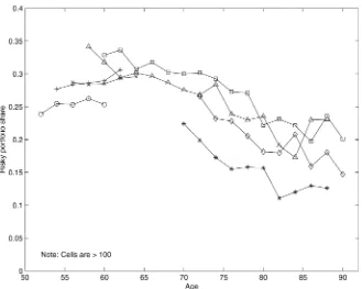
Classic portfolio choice theory as stated by Merton (1969, 1971) and Samuelson (1969) recommends that as long as stock returns display no mean reversion, investors should place a con-stant share of their wealth in risky assets regardless of their ages or time horizons. This contrasts both with traditional personal investment advice, which proposes that risky portfolio shares should be 100 minus the investor’s age (Malkiel 1999), and with empirical evidence on the actual portfolio behavior of indi-viduals, which generally exhibits declining risk taking through age, even after retirement (Guiso, Haliassos, and Jappelli 2002; Ameriks and Zeldes 2004). Figure 1 depicts this relationship using data from several waves of the Health and Retirement Study (HRS) between 1992 and 2000. These patterns could be produced by any combination of age, cohort, and time effects. As has been widely remarked, identification of these separate effects can only formally derive from restrictions in longitu-dinal data. There is no universal agreement in the literature, but modeling age and time effects is standard (Heaton and Lucas 2000a; Ameriks and Zeldes 2004; Cocco, Gomes, and Maenhout 2005).
There have been numerous efforts to reconcile theory with empirical patterns since Merton and Samuelson published their results. Many of the insights accumulated since then provide compelling explanations for the vast differences in portfolios that we see between young and old investors, but few can ex-plain continued declines in risk taking with age after retire-ment. Much research has focused on the role of labor income (Jagannathan and Kocherlakota 1996; Elmendorf and Kimball 2000; Viceira 2001; Campbell and Viceira 2002; Cocco et al. 2005). If labor income is a hedge against financial risk, then young workers should invest their assets more riskily than old retirees. But this rationale best explains relatively abrupt changes in portfolio choice leading up to retirement, not the continuous declines with age after retirement seen in Figure 1.
Examining data from the Study of Assets and Health Dy-namics Among the Oldest Old (AHEAD), I show that retired individuals view their health as risky, and they appear to de-crease their exposure to financial risk to hedge against it. Be-cause health tends to become riskier with age, the presence of undiversifiable health risk may explain why investors decrease their financial risk with age even after retirement. Exactly how risky health prompts investors to hedge in this manner re-mains somewhat unclear. There are two main candidates: ei-ther the specter of out-of-pocket medical expenditures looms
large, even for Medicare beneficiaries, or retired investors an-ticipate that adverse health shocks will raise their marginal util-ities, presumably by impeding home production. I show that the evidence seems to fit the latter explanation better, but both chan-nels are potentially important. The presence of spouses and in-tended bequests, whereas could represent the promise of infor-mal care arrangements, appear to decrease portfolio responsive-ness to risky health, whereas additional health insurance does not. Point estimates suggest that risky health may explain 20% of the age-related decline in financial risk taking after retire-ment.
2. BACKGROUND AND THEORETICAL MOTIVATION
A number of previous efforts have explored the relationship between health and financial decision making. There is a well-established literature on precautionary saving, and several ar-ticles examine how future health expenditures may increase saving (Hubbard, Skinner, and Zeldes 1994; Palumbo 1999; Dynan, Skinner, and Zeldes 2004). Others have examined port-folio choice relative to health. Guiso, Jappelli, and Terlizzese (1996) found that Italian households headed by individuals who spent more days sick tended to hold safer financial portfolios, even after controlling for many other variables. Rosen and Wu (2004) showed a robust association between fair or poor health status and safe portfolios in the Health and Retirement Study.
2.1 Health and Planning
There are several reasons why health might affect financial decisions. First, future health shocks can trigger out-of-pocket medical spending which absorbs financial wealth and raises its marginal utility. The precautionary saving motive, or “pru-dence” (Kimball 1990), prompts individuals to acquire more wealth to offset this background risk. Similarly, any risk that leads to such precautionary saving should also lower the de-mand for risky assets, or result in “temperance” (Kimball 1992; Elmendorf and Kimball 2000). In this view, health expendi-tures constitute a type of undiversifiable background risk that prompts safer portfolios (Heaton and Lucas 2000b). Pratt and
© 2008 American Statistical Association Journal of Business & Economic Statistics October 2008, Vol. 26, No. 4 DOI 10.1198/073500107000000287
472
Figure 1. Age profiles ofαin five HRS and two AHEAD waves. Data are from the 1992, 1994, 1996, 1998, and 2000 HRS waves, and the 1993 and 1995 AHEAD waves. Each age range is labeled with its endpoint. Risky portfolio shares are constructed as the ratio of risky financial assets to total financial assets. Total financial assets include IRA/Keogh accounts; stocks and stock mutual funds; checking, saving, and money market accounts; CDs, government savings bonds, and Treasury bills; and corporate and other government bonds and bond funds. Risky financial assets are defined as the sum of the risky portion of IRA/Keogh accounts plus stocks and stock mutual funds. The risky portion of IRA/Keogh accounts is set at half of total IRA/Keogh balances except in the 1998 and 2000 HRS, when available data indicated a 60–40 split. ( 2000; 1998; 1996; 1995; 1994; 1993; 1992).
Zeckhauser (1987) showed that such “proper risk aversion” holds for most commonly used utility functions, and Gollier and Pratt (1996) added that even mean-zero independent risks generate “risk vulnerability,” which induces more risk-averse behavior toward any other risk.
The second reason why health could affect financial deci-sions is if health status directly affects marginal utility, or put another way, if the cross partial derivative of utility is nonzero. If the cross partial is positive, then health and consumption may be called Frisch or Edgeworth–Pareto complements (Samuel-son 1974), and an adverse shock that lowers health will also decrease marginal utility. In such a world, individuals expect-ing health shocks should save less and invest their savexpect-ings more riskily, because health shocks are like a hedge against risks to future consumption. The reverse is true if the cross partial is negative: health shocks raise the marginal utility of consump-tion and compound risks to future consumpconsump-tion.
A third potential channel is through life span or planning horizon. Health and mortality are related, so risky health should imply risky survival. But it is less clear what effect longevity risk has on financial planning. In a model with no labor income or annuities, an uncertain date of death prompts individuals to save to hedge against the risk of living too long. But life-span uncertainty also reduces the marginal utility of holding wealth because there is a chance of dying before it can be spent. As discussed by Kalemli-Ozcan and Weil (2002), this may reduce saving if retirement is late enough or can be postponed.
A related question is whether the expected length of the time horizon should matter for portfolio behavior. All things equal,
advancing age leaves less time remaining before death, which some may argue is reason enough to invest more safely. But if utility is time-separable and exhibits constant relative risk aver-sion (CRRA), and if asset returns are independently and iden-tically distributed, without any mean reversion, then investors facing a planning horizon of any length ought to behave “my-opically,” maintaining the same optimal risky portfolio share through time (Merton 1969; Samuelson 1969). Modern port-folio choice theory admits there may be mean reversion in as-set returns, and that labor income may alter decisions prior to retirement, but it typically rejects the notion that a shortening planning horizon alone is a reason to reduce risk (Jagannathan and Kocherlakota 1996; Campbell and Viceira 2002). Cocco et al. (2005) showed that an investor with a defined-benefit pen-sion should optimally shift toward more risk with increasing age, as financial wealth diminishes relative to pension wealth through life-cycle dissaving.
Several other elements are related to survival and possibly to portfolio choice. Cocco et al. (2005) found that a bequest mo-tive can in theory make safe assets somewhat more attracmo-tive later in life, but the risky share hardly declines with age even in their simulations with the strongest bequest motive. Hurd (2002) uncovered little evidence that bequest motives are im-portant in describing portfolio choice among elderly Americans in the AHEAD, perhaps reflecting the lack of empirical support for intended bequests (Hurd 1989). Household composition is another factor related to financial risk taking (Bertaut and Starr-McCluer 2002; Rosen and Wu 2004), and trends in health and
survival may be correlated with household structure. An emerg-ing theme in this article is that bequests and household structure should be related to the sign of the cross partial, as I discuss in greater detail later.
It is unclear which of these channels are important in de-scribing the age trajectory of portfolio choice, or if all are. Previous research suggests the two most likely candidates are health expenditures and state-dependent utility. Although out-of-pocket medical expenditures do not appear to be large on average (Smith 1999), they are autocorrelated and occasion-ally catastrophic (French and Jones 2004). Cocco et al. (2005) modeled portfolio choice with health spending shocks ranging up to 75% of retirement income using numerical techniques. They found that financial risk taking actually increases slightly with age after retirement, owing to more rapid depletion of non-pension wealth, but they did not account for the persistence of health expenditure shocks. Rosen and Wu (2004) found that fair or poor health status is associated with safer financial portfolios regardless of health insurance status or out-of-pocket medical expenditures including prescription drugs. Apparently some-thing about poor health other than the risk of current and future health expenditures is affecting portfolio choice.
2.2 The Nature of the Cross Partial
A negative cross partial could explain the results of Rosen and Wu (2004) if poor health today were predictive of poor health, and thus higher marginal utility, in the future. Health insurance typically reimburses the costs of medical goods and services rather than simply paying cash in the unhealthy state, so risk associated with a negative cross partial could impinge regardless of insurance status. Unfortunately, evidence on the sign of the cross partial is mixed. Viscusi and Evans (1990) found that chemical workers expect their marginal utilities to decline in bad health, or that the cross partial is positive. Evans and Viscusi (1991) reported that temporary health conditions like burns and poisonings seem not to affect the marginal util-ities of surveyed adults. Lillard and Weiss (1997) showed that adverse health shocks apparently raise the marginal utility of consumption among elderly households, or that the cross par-tial is negative, which induces transfers from the healthy to the sick partner and provides an extra precautionary motive for sav-ing.
It is unclear what may be driving the different results across these empirical studies; they use completely different data and focus on individuals of vastly different ages who face com-pletely different types of health conditions. The cross partial could change sign during the life course, if the reaction to spe-cific health conditions varied by health status or prior exposure. The cross partial could also be different for different health con-ditions, which can also be age-specific.
The cross partial should be positive for conditions that sim-ply impede the enjoyment of consumption, for example, when a common cold inhibits going to the theater or taking a vaca-tion. Debilitating illness may do likewise but would surely also impede nonmarket production of essential goods and services, which should raise the demand for funds to replace them. In addition to lowering the marginal utility of a vacation, a broken hip may require taking a taxi instead of walking, for example,
or hiring a maid instead of cleaning. Depending on the value of lost home production relative to the value of foregone recre-ational spending, the net cross partial for debilitating shocks may be positive or negative. If it were negative, the presence of family members should partially hedge this risk to essential nonmarket production, because their labor could make up the difference. Families may also affect how an individual’s recre-ational enjoyment of goods and services changes with his or her health, but it is less clear how.
The findings of Cocco et al. (2005) and Rosen and Wu (2004) with regard to health expenditures and insurance suggest it is worthwhile to examine how a negative cross partial could theo-retically affect portfolio choice. To motivate my subsequent em-pirical analysis, I present and discuss an analytical solution to a log-linearized model of portfolio choice that I have developed elsewhere (Edwards 2007). I leave to future efforts a more de-tailed examination of a full life-cycle model of portfolio choice with calibrated risks of future health shocks, health expendi-tures, uncertain life spans, bequests, and household composi-tion.
3. PORTFOLIO CHOICE AND THE CROSS PARTIAL
Following Picone, Uribe, and Wilson (1998), suppose retired investors have nonseparable Cobb–Douglas tastes over health,
Ht, and consumption,Ct:
Ut(Ct,Ht)=
(CtψHt1−ψ)1−γ
1−γ , (1)
whereψ∈(0,1) andγ >0. There are two states of nature, healthiness and unhealthiness. Healthy investors are endowed with health and cannot purchase any more but perceive a peri-odic risk,πh∈(0,1), of becoming permanently unhealthy.
Un-healthy investors must purchase their health each period. Both investors may allocate their wealth into risky or risk-free assets, which pay returns ofr∼N(μr, σr2)andrf, and there is no labor
income.
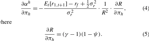
As shown by Edwards (2007), this problem can be solved using the log-linearization techniques of Viceira (2001) and Campbell and Viceira (2002). Healthy investors who perceive a level of periodic health riskπhwill invest a shareαtof their
wealth in the risky asset that is given by
αt=
Et[rt+1] −rf+12σr2
R(ψ, γ , πh)·σr2
, (2)
whereEt[rt+1] −rf is the equity risk premium,σr2is the
vari-ance in risky asset returns, and
R(ψ, γ , πh)=1−(1−γ )ψ+(1−ψ )πh (3)
is an expression for what we can call the investor’s effective risk aversion, a function of the preference parameters and perceived health risk. When the investor does not care about health,ψ=1 andR=γ, and (2) reduces to the classic Merton–Samuelson result.
The implications of this model for portfolio choice when health is risky depend on the sign of the cross partial deriva-tive of utility,∂2U/∂H∂C, which is determined by the magni-tude ofγ. Whenγ∈(0,1), the cross partial is positive; when
γ=1, the cross partial is zero; and whenγ >1, the cross par-tial is negative. As long as health affects utility, (2) and (3) re-veal that when the cross partial is negative, investors will reduce their risky portfolio shares in response to increasing health risk; when it is zero, they will not change their portfolio shares; and when it is positive, they will increase their risk taking in re-sponse to health risk:
When the cross partial is negative, γ >1 and future health shocks will raise marginal utility. In the model, health riskπh
raises effective risk aversion, R(·), and inspires less risk tak-ing. If instead the cross partial is positive, investors will in-crease their risky portfolio share as health risk inin-creases. Health shocks are actually a form of implicit insurance in that setting, because the demand for funds is diminished when sick, and ef-fective risk aversion is lower. If the cross partial is zero, then health shocks do not affect the marginal utility of consumption, and investors will not alter their portfolio strategies in response to risky health status.
The importance of the cross partial to the analytical result is simultaneously limiting and interesting. As I discussed in the previous section, the empirical literature is split on the sign of the cross partial, with the nature of the health shock a poten-tially important variable. But the notion that health may af-fect portfolio choice directly through the utility function is a new insight. To be sure, any shock that changes marginal utility will also affect intertemporal choice. Health is special because it represents truly undiversifiable risk, and it varies systemati-cally over the life cycle. Many shocks threaten to absorb wealth and thus raise marginal utility. But if contingent claims markets are complete, individuals should be able to write contracts that diversify away many such risks. Health, unlike cash, certainly cannot be insured in-kind. Contracts that directly deliver cash contingent on the health state are typically limited to life insur-ance, which conditions on a very special health state.
But expenditures on health can be insured, and we know that many Americans face significant gaps in health insurance cov-erage. A noteworthy and unfortunate absence in the solution to this log-linearized model is any role for the risk of future health expenditures. They do induce precautionary saving in the model, but as long as they are uncorrelated with financial market risk, they have no effect on portfolio choice. Given the breadth of theoretical and empirical literature revealing portfo-lio responses to background risk, this seems like a result that is specific to the log-linearization technique and not a general one.
Unraveling the effects of risks to health status versus risks of out-of-pocket health expenditures is a worthwhile future en-deavor. Here, I instead explore the empirical relationship be-tween self-perceived risks to health and risky portfolios to as-sess the scope for a model of risky health to provide insights into actual behavior. I calibrate the solution of the log-linearized model of portfolio choice to aggregate data and use those find-ings as motivation and guide to interpreting microeconometric results.
4. AGGREGATE PATTERNS AND MODEL CALIBRATION
4.1 The Data
Figure 1 shows seven cross-sectional age profiles of risky portfolio shares between 1992 and 2000, averaged within two-year age groups. The risky portfolio share,α, is defined as risky financial wealth, such as stocks and stock mutual funds, divided by total financial wealth, which also includes safer instruments like bills, bonds, and bank accounts. I observe risky shares dur-ing five waves of the Health and Retirement Study (HRS) and two waves of its sister dataset, the Study of Assets and Health Dynamics Among the Oldest Old (AHEAD), and I connect ob-servations for each wave. A clear downward trend in financial risk taking by age is apparent. Investors of working age, or younger than 65, generally have α’s between .25 and .35, or about.30 on average. Older investors are clustered between.10 and about.25, or perhaps.175 on average. Ameriks and Zeldes (2004) reported similar levels based on Surveys of Consumer Finances and TIAA-CREF data.
It is more difficult to measure risks to health. Researchers have imputed future health expenditure risks from cross-sectional data (Lillard and Weiss 1997; Palumbo 1999), panel data on tax returns (Hubbard et al. 1994), or more recently from rich panel data in the HRS/AHEAD surveys (French and Jones 2004). In this article, I take a simpler approach that explores individuals’ actual perceptions of risk. A question contained in the 1993 and 1995 waves of the AHEAD allows me to examine the self-reported probabilities of future health events expected by retirees rather than imputations of likely future events. Dur-ing these waves, individuals over age 70 were asked to state the probability that “medical expenses will use up all [their house-hold] savings in the next five years.” Respondents indicated a risk of this future event, a probability I will labelπhand refer to
as health risk, that averaged between 25% and 30%. Although the data exhibit much pooling at focal responses like 0, 50, and 100, we know that the HRS expected-survivorship questions also exhibit pooling but still are good indicators of health and mortality (Hurd and McGarry 1995, 2002). So it is likely that the answers to this AHEAD question reflect legitimate assess-ments of risks of health expenditures.
These perceptions of catastrophic or near-catastrophic risks to out-of-pocket health expenditures are arguably also measur-ing self-perceived catastrophic risks to health status. To be sure, these two sets of outcomes, one concerning health expendi-ture and the other health status, may not perfectly overlap. The AHEAD question will mismeasure risk to health status by miss-ing any cheap but debilitatmiss-ing shocks while pickmiss-ing up expen-sive but relatively benign conditions. Because the latter, or a false positive, is likely to be a rare occurrence at older ages, the AHEAD variable may understate the true catastrophic risks to health status.
Another limitation is that we do not know how households younger than those in the AHEAD would have answered this question. The younger HRS cohorts were only asked about the probability of health limiting their work activity. Thus we can only measure self-perceived risks to health at older ages, and we can only guess at how they evolve over the life cycle.
4.2 Model Calibration
Given that we observe an average self-perceived health risk of about πh = .25 among AHEAD respondents, we
might conjecture that the average increase over the life cy-cle in πh could be as much as .25. Suppose all of the
ob-served age-related decline in the risky portfolio share, α, from .3 to .175, were due to that increase in πh. Then a
very simple estimate of the regression coefficient on health risk in a multivariate linear regression of portfolio shares is ∂α/∂πh≈α/πh=(.3−.175)/.25= −.5.
Now consider our stylized analytical model of portfolio choice under health risk with Cobb–Douglas preferences over consumption and health. We can recover an estimate of∂α/∂πh
from this model by calibrating (2) using moments of aggre-gate financial data, observed risky portfolio shares, and obser-vations and assumptions aboutπh. There are three unknowns:
the health risk faced by younger investors, and the two pref-erence parameters:γ, which governs the overall utility curva-ture and also determines the sign of the cross partial, and ψ, the utility weight on consumption. Researchers typically make assumptions about the preference parameters (Hubbard et al. 1994; Picone et al. 1998; Heaton and Lucas 2000b). But be-cause the sign of the cross partial depends onγ, it seems more appropriate in this case to recover the preference parameters from assumptions about the health risk faced by younger in-vestors. We can write down two versions of (2), one for young investors and one for old investors, and then solve for the two unknown preference parameters assuming some level of health risk faced by young investors.
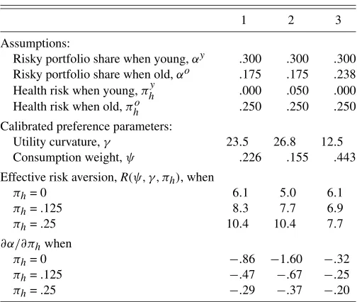
Table 1 displays means and standard deviations of the finan-cial parameters as reported by Campbell, Lo, and MacKinlay (1997) and revealed from HRS and AHEAD data on portfo-lio shares in Figure 1. In the middle of Table 2, I list several combinations of the preference parameters, γ andψ, that are consistent with the financial parameters and with assumptions about health risk among younger investors,πhy, and the amount of the age-related decline in portfolio shares to be explained by the model. At the bottom of the table, I report the levels of ∂α/∂πhthat are consistent with these preference parameters.
If we assume that all of the age-related decline in risky port-folio shares is due to health risk, πh, and if we assume that
younger investors face πh=0, then the model requires that γ=23.5 andψ=.226. This is shown in the first column of Ta-ble 2. The levels of effective risk aversion implied byγ=23.5 and ψ=.226 for various levels of health risk are between 6.1 and 10.4, which are consistent with the range explored by Heaton and Lucas (2000b). The marginal effects of health risk on the risky portfolio share vary between−.86 for young in-vestors facing virtually no risk and −.29 for retired investors facing πh=.25. The consumption weight, ψ, is small
com-pared with that assumed by Picone et al. (1998), who chose ψ=.6, and it implies rather unrealistically that investors in the unhealthy state would spend 77% of their income on health. Health gets such a large utility weight because nothing else in the stylized model can explain the rather large age-related decline inαfrom .3 to .175 other than health. Health gets an even larger utility weight in the second column, where I set the unknown level of health risk among young investors to
Table 1. Moments of financial data
Mean stock returns,Et[r1,t+1] .0601
Risk-free return,rf .0183 Variance in stock returns,σr2 .0315 Risky portfolio shares among:
Working-age households,αy .300 Retired households,αo .175
NOTE: Rows 1–3 are taken from table 8.1 in Campbell et al. (1997). Stock returns are measured as annual log real returns on the S&P 500 index since 1926 and a comparable series prior to 1926. Risk-free returns are annual log real returns on 6-month commercial paper bought in January and rolled over in July.σr2=Vart[r1,t+1−rf]. Rows 4–5 are
average risky portfolio shares across households by age based on data in the HRS and AHEAD datasets shown in Figure 1.
πhy=.05 instead of zero. Because we are still forcing the model to explain a decline of 12.5 percentage points in the risky port-folio share with changing health risk, a smaller change inπh
requires a larger utility weight on health to explainα. In the third column, I ask the model to explain only half the drop inα, or the 6.2 percentage points from .3 to .238, and the calibrated consumption weight rises to a more reasonableψ=.443. The marginal effect of health risk varies between−.2 and−.32 de-pending on its level.
With a negative cross partial derivative, so that the need for funds is greater in the unhealthy state, the analytical model can reproduce observed moments in the financial data and trends in portfolio behavior by age after retirement. The calibration exercise reveals estimates of the marginal effect of health risk on portfolio choice,∂α/∂πh, that average about −.3 for
indi-viduals facing levels of health risk around πh=.25, such as
AHEAD respondents. But although it is possible to explain all the age-related decline in risky portfolio shares using the model, the associated calibrated results are less than fully convincing because the model places an unrealistically heavy weight on health in utility. This suggests there are other factors affecting
Table 2. Calibration of the portfolio choice model with Cobb–Douglas preferences over health and consumption
under various assumptions NOTE: This table reports calibrated parameters of a model of portfolio choice under Cobb–Douglas preferences shown in (1). The calibration proceeds by setting values for the top four variables and solving the nonlinear system defined by (2) forγandψ.
portfolio choice that the model is missing, and that I should account for a range of covariates in the empirical analysis of microdata.
5. MICRO–LEVEL TESTS OF THE HEALTH RISK MODEL
5.1 The Data
To further explore portfolio choice and health risk, I ex-amine microdata from the AHEAD dataset. The AHEAD fol-lows roughly 8,200 individuals in 6,000 households selected to represent the birth cohorts born in 1923 and earlier (Juster and Suzman 1995). First interviewed in 1993, the panel was reinterviewed in 1995 and then merged with its sister study, the HRS, in 1998. Only in the 1993 and 1995 waves of the AHEAD were any individuals asked the question about the like-lihood of catastrophic health expenditures that I discussed ear-lier. Each respondent in the household could answer that ques-tion, whereas wealth variables are defined only at the level of the household. In the analysis that follows, I assign the house-hold’s wealth and portfolio shares to both individuals when present, and I condition on household composition.
I obtained most of the variables from version E of the RAND HRS dataset, which is a cleaned, more user-friendly version of the original source data. I merged the RAND data with the orig-inal AHEAD datafiles in order to obtain the measure of self-perceived risks to health and several other variables.
5.2 Empirical Strategy
I posit the following linear regression model of the risky port-folio share observed for individualiat timet:
α(i,t)=β0+D(t)+β(i)+βhπh(i,t)
+
k
βkxk(i,t)+ǫ(i,t), (6)
whereβ0 is a constant that measures aggregate financial
pa-rameters like the equity risk premium,D(t)is a time dummy that picks up changes in aggregate financial parameters,β(i)is an individual (household) random effect that I include as a ro-bustness check, πh(i,t)is self-perceived health risk, and the
xk(i,t)’s are other covariates that matter for portfolio choice,
which I discuss below. Including a time dummy represents an identifying assumption that there are age and time effects in portfolio choice and no cohort effects. As I acknowledged ear-lier, there is no a priori reason to make this assumption. Rather, it reflects the precedent set by Heaton and Lucas (2000a), Cocco et al. (2005), and Ameriks and Zeldes (2004), the latter of whom argued that patterns in panel data do not support cohort effects.
As is typical, empirical measures of risky portfolio shares exhibit significant pooling atα=0 and 1, and many even lie outside the unit interval. The basic Merton–Samuelson frame-work suggests that portfolio shares should lie between 0 and 1 given the financial parameters listed in Table 1, unless the indi-vidual has extremely small or negative effective risk aversion. Practically speaking, a variety of other influences may prompt investors to hold either all or none of their financial wealth in
risky assets, such as nonparticipation in equity markets, large holdings of risk-free nonfinancial assets, executive compensa-tion in the form of company stock, and so on. Measurement er-ror could also push the risky portfolio share too high or too low; financial wealth in the HRS/AHEAD surveys is imputed using hot-deck techniques for a large number of households (Juster and Suzman 1995). Following Guiso et al. (1996), Rosen and Wu (2004), and others, I use the tobit model to estimate (6), with limits at both truncation points:α=0 and 1.
5.3 Portfolio Choice Covariates
An assortment of other variables belong in the empirical model even though they do not formally appear in the stylized theoretical model. The inclusion of many of these can be jus-tified by their association with preferences for risk, which are parameters of the theoretical model that are not directly mea-surable.
Wealth directly affects tastes for risk if utility does not dis-play constant relative risk aversion. The AHEAD measures sev-eral types of wealth, including financial wealth, housing, and vehicular assets, so I can easily control for them. Some types of wealth are interesting for life-cycle behavior even when util-ity is CRRA. Annuities and defined-benefit pensions like Social Security pay out some fixed amount each period, sometimes in-dexed to inflation, conditional only on survival. As mentioned earlier, life-cycle dissaving of nonpension wealth through age will increase the relative size of this essentially risk-free pen-sion wealth in the overall portfolio, incentivizing greater risk taking. I construct Social Security wealth and defined-benefit pension wealth for the AHEAD cohort utilizing the techniques of Poterba, Rauh, Venti, and Wise (2003). I use cohort life ta-bles for men and women produced by the Social Security Ad-ministration (Bell and Miller 2005) to weight future income flows. These are also discounted by a real rate of 3% in the case of Social Security benefits, which are indexed against in-flation, and 6% for defined-benefit pensions, which typically are not. If both members of a couple remain alive, the household receives both respondents’ individual Social Security benefit. When only one member of the couple is alive, the household receives the maximum of the two benefits.
Following Rosen and Wu (2004) and others, I also include as covariates current health status, education, sex, race and ethnic-ity, household composition, the number of surviving children, and age. Rosen and Wu found that portfolio shares are robustly associated with a binary measure of fair or poor self-reported health status among younger members of HRS households, so I include the same variable here. Education may affect portfo-lio choice by enhancing financial knowledge about the benefits of diversification or the equity premium. Sex, race, and eth-nicity typically matter because these subgroups may differ in their perceptions of and tolerances for risk. Household compo-sition and the number of surviving children may affect portfolio choice through the bequest motive, and they may also represent a means to spread risk informally. In particular, households of sufficient size may be able to hedge idiosyncratic risks to home production. This is a particularly interesting channel to explore because a negative cross partial could stem from debilitating health shocks that threaten home production.
Age may be a proxy for risk preferences, and traditional in-vestment advice specifies portfolio shares as a linear function of age (Malkiel 1999). With the AHEAD data, I can also con-struct a variable that measures a person’s expected remaining years of life by transforming self-reported survivorship prob-abilities in the appropriate way. Because each respondent pro-vides only one probability, I assume a linear survivorship sched-ule with everyone dying by age 110. If the time horizon matters for portfolio choice, expected remaining years of life should have a more robust effect than age, which is at best a rough proxy for a particular individual’s time horizon.
The richness of the AHEAD datasets also allows me to con-trol for stated bequest motives and several types of health in-surance. This parallels Rosen and Wu, who examined portfolio choice among the original HRS cohort. They were asked sim-ilar questions about the probability of leaving any bequest, the presence of additional health insurance, long-term care insur-ance, and life insurance. All of these may affect financial deci-sion making.
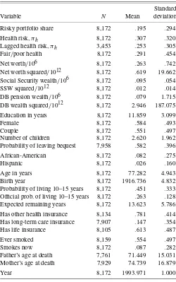
Summary statistics for the variables in the pooled AHEAD dataset are presented in Table 3. The average risky portfolio share across both years is .195, with a high standard deviation. I have manually truncated portfolio shares at 0 and 1 to be con-sistent with the tobit regressions later. The average health risk in the two-year pooled dataset is .307, whereas it is .253 in 1993 for individuals who answered it both years. I include lagged health risk because it is a useful instrument. Future health risk is thus relatively high, and almost 30% of the pooled sample re-port fair or poor health. Household finances vary considerably across the sample. Net worth, which is the sum of the values of housing and other real estate, vehicles, businesses, financial as-sets, minus the sum of all debts, averages $263,000 and also dis-plays much variability. Social Security wealth amounts to only about $95,000 per household, but it is much more evenly dis-tributed. Defined-benefit pension and annuity wealth is smaller still, at $79,000 per household, with an extremely high standard deviation.
Almost 60% of the sample is female, but over half of all in-dividuals are in couple households. Children are common, and family size varies considerably. The average self-reported prob-ability of leaving any bequest at all is nearly 60%. Survivorship probabilities average 45%, almost 20 percentage points higher and more variable than suggested by official period life tables. Expected years of life, which I compute from self-reported sur-vivorship, therefore average a relatively high 13.6 years with a standard deviation of 5.8 years. A large share of individu-als, over 75%, report health insurance coverage in addition to Medicare. Barely 15% have private long-term care insurance. Over 60% have life insurance. The bottom of the table lists variables I use as instruments for health risk. There is con-siderable variation in past and even present smoking behav-ior, as well as in the life spans of parents, and all of these variables should determine expectations about future health events.
5.4 Results
5.4.1 Baseline Tobits by Household Composition. Cali-bration of the model to aggregated data suggests that the
coef-Table 3. Means and standard deviations in the pooled AHEAD dataset
Standard Variable N Mean deviation Risky portfolio share 8,172 .195 .294 Health risk,πh 8,172 .307 .320 Lagged health risk,πh 3,453 .253 .305
Fair/poor health 8,172 .291 .454 Net worth/106 8,172 .263 .742 Net worth squared/1012 8,172 .619 19.662 Social Security wealth/106 8,172 .095 .054 SSW squared/1012 8,172 .012 .014 Probability of leaving bequest 7,958 .582 .396 African-American 8,172 .082 .275 Hispanic 8,172 .026 .160 Age in years 8,172 77.282 4.943 Birth year 8,172 1916.736 4.832 Probability of living 10–15 years 8,172 .451 .333 Official prob. of living 10–15 years 8,172 .263 .128 Expected remaining years 8,172 13.623 5.786 Has other health insurance 8,134 .781 .414 Has long-term care insurance 7,907 .147 .354 Has life insurance 8,105 .613 .487 Ever smoked 8,159 .554 .497 Smokes now 8,172 .087 .282 Father’s age at death 7,761 71.449 15.031 Mother’s age at death 7,929 74.739 16.879 Year 8,172 1993.971 1.000
NOTE: Data are pooled observations of individuals in the 1993 and 1995 waves of the Study of Assets and Health Dynamics Among the Oldest Old (AHEAD). Wealth is a house-hold variable. Risky portfolio shares are constructed as the ratio of risky financial assets to total financial assets. Total financial assets are IRA/Keogh accounts plus stocks and stock mutual funds plus checking, saving, and money market accounts plus CDs, government savings bonds and Treasury bills plus corporate and other government bonds and bond funds plus other financial assets, minus debts. Risky financial assets are defined as the sum of the risky portion of IRA/Keogh accounts plus stocks and stock mutual funds. The risky portion of IRA/Keogh accounts is set at half of total IRA/Keogh balances. Total net worth is total (net) financial assets plus the value of real estate, businesses, and vehicles. Social Security wealth and defined-benefit (DB) pension wealth are the expected present value of the household’s future Social Security income or pension/annuity income, constructed as in Poterba et al. (2003) and described in the text. Expected remaining years of life is derived from the self-reported survivorship probability as described in the text. The official probability of living another 10–15 years is taken from NCHS period life tables.
ficient on health risk should be negative,βh<0, in the range
of −.2 to −.4 for the AHEAD cohort. The first row of Ta-ble 4 presents estimates ofβhfrom two-limit tobit regressions
of portfolio shares using various subsets of the pooled AHEAD data characterized first by household status and then by year. Subsequent rows list estimated coefficients for the other covari-ates. The average risky portfolio share,α, in each subsample appears at the bottom of each column, followed by regression diagnostics.
Over all households in the pooled sample, the marginal as-sociation between health risk and the risky portfolio share is βh= −.138, as shown in the first column. This is a smaller
Table 4. Tobit regressions of portfolio shares using pooled AHEAD data with varying household composition and year
By household composition By year, all HH’s Variable All HH’s Singles only Couples only 1993 only 1995 only Health risk,πh −.138* −.220* −.072* −.126* −.133*
(.023) (.042) (.027) (.036) (.029)
Fair/poor health −.073* −.079* −.062* −.074* −.065*
(.016) (.031) (.019) (.025) (.021)
Net worth/106 .221* .348* .273* .527* .166*
(.014) (.034) (.019) (.036) (.015)
Net worth squared/1012 −.006* −.008* −.014* −.033* −.004*
(.000) (.001) (.001) (.004) (.001)
Social Security wealth/106 1.441* 2.195* 1.057* 1.561* 1.711*
(.372) (.997) (.416) (.629) (.461)
SSW squared/1012 −2.071 −2.409 −1.409 −3.596 −2.657
(1.300) (5.309) (1.374) (2.328) (1.536)
DB pension wealth/106 .088 .105 .118* .439* .088
(.049) (.197) (.056) (.153) (.054)
DB wealth squared/1012 −.001 −.061 −.001* −.350* −.001
(.000) (.049) (.001) (.105) (.000)
Education in years .046* .054* .038* .038* .045*
(.003) (.005) (.003) (.004) (.003)
Female −.048* −.059 −.042* −.041 −.051*
(.014) (.031) (.016) (.022) (.019)
Couple .082* .101* .042
(.017) (.026) (.022)
Number of children −.013* −.025* −.008 −.013* −.012*
(.004) (.007) (.004) (.006) (.005)
African-American −.331* −.372* −.297* −.338* −.311*
(.032) (.055) (.042) (.050) (.042)
Hispanic −.196* −.227* −.188* −.204* −.188*
(.052) (.099) (.060) (.084) (.064)
Age −.010* −.008* −.010* −.011* −.007*
(.002) (.003) (.002) (.002) (.002)
Expected remaining years .001 .001 −.000 .000 .001
(.001) (.003) (.002) (.002) (.002)
Year .062* .095* .041*
(.007) (.013) (.008)
E[α] .20 .15 .23 .18 .22
Observations 8,172 3,668 4,504 4,206 3,966
χ2-statistic 1,847 693 949 967 922
Prob> χ2 .00 .00 .00 .00 .00
NOTE: Standard errors are in parentheses. Asterisks denote significance at the 5% level. Data are pooled observations of individuals in the 1993 and 1995 AHEAD surveys, except for columns 4 and 5, which include only one wave each as a robustness check. The dependent variable isα, the risky portfolio share, constructed as described in the text and in the notes to Table 3. All regressions are tobits with limitsα=0 andα=1, and all include a constant term (not shown). Health risk,πh, is the self-assessed probability that medical expenses will
use up all household savings in the next five years, expressed as a fraction, 0 to 1. Health status may be reported as excellent, very good, good, fair, or poor. Net worth is total assets, including real estate, business, vehicular, and financial assets, minus debts. Social Security wealth and defined-benefit (DB) pension wealth are constructed as described in the text and in the notes to Table 3. Education is measured in years. Couple, African-American, and Hispanic are indicator variables. Kids is the number of surviving children. Remaining years are the expected number of remaining years before death as inferred from the individual’s subjective survivorship response.
coefficient than predicted by the calibration exercise and one that attributes about 3 percentage points, or about one quar-ter, of the 12.5% decline in the risky portfolio share to age-related increases in health risk. Other coefficient estimates in the first column generally match our priors and the results in previous literature. Fair or poor health reduces the risky share by about 7 percentage points, which is roughly in line with the results of Rosen and Wu (2004), who examined the younger HRS cohort. It is worth remarking that even after conditioning on current health status, health risk is still significantly associ-ated with safer portfolio shares. All three types of wealth—net worth, Social Security wealth, and defined-benefit (DB)
pen-sion wealth—matter for portfolio choice. Of the three, Social Security wealth has the largest impact on portfolio choice, but it also varies the least within the sample. I also tested alter-native definitions of net worth such as financial or nonhous-ing net worth and found results varied little. Education is ro-bustly associated with riskier portfolios, whereas being female, African-American, or Hispanic is associated with safer port-folios. The effect of age is negative and fairly robust, averag-ing about −.01 across the first three columns. This is consis-tent with the standard investment advice provided by Malkiel (1999), who suggested declines of one percentage point per year of age. Although its coefficient is at least positively signed,
expected remaining years of life have no significant impact, per-haps because the variable is noisy.
Table 4 reveals strong effects of household composition on portfolio choice. The coefficient on the couple dummy in the first column is positive and significant, showing that the pres-ence of a spouse or partner is associated with riskier portfolios. But the number of surviving children does not provide the same kind of hedge; that coefficient is negative and significant, even after controlling for wealth. To explore the effects of house-hold composition further, I split the sample into couples and singles and reestimate in the next two columns. This reveals a significantly stronger effect of health risk among singles, with βh= −.220, than among couples, for whomβh= −.072, with
both coefficients significant at 5% level and displaying nonover-lapping confidence intervals. Not only do couples take on more financial risk than singles, which is a standard finding; they also view risks to health as less threatening. This is consistent with a negative cross partial deriving from the need to replace home production when sick. Under those circumstances, the presence of a spouse or partner is a direct hedge against health risk, whereas a single must replace home production with market production when sick.
The fourth and fifth columns explore conditioning on one or the other sample year rather than household composition, to ex-amine the temporal variation in the pooled dataset. The wealth questions and imputations have evolved with the survey, and we would like to know whether the more recent data are bet-ter. Few notable differences emerge, which suggests there is no significant change in quality between the two waves. The av-erage risky portfolio share among this large age cohort jumped from .18 to .22 between 1993 and 1995, probably spurred by the roughly 25% cumulative rise in stock indexes during this period.
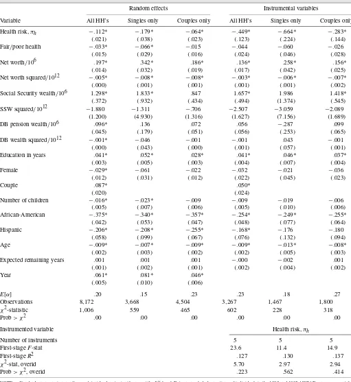
5.4.2 Tobits With Random Effects. The first three columns in the left panel of Table 5 add household random effects to the tobit regressions as a robustness check. Fixed effects are less practical in a short panel with relatively little time variation, and they are more difficult to estimate in a truncated regression model (Honore 1992). Rosen and Wu (2004) and van Soest and Kapteyn (2006) both used random effects in explaining portfo-lio behavior in several waves of the HRS. Including household random effects using both years of data does not significantly alter the results. Estimated coefficients on health risk become smaller in magnitude by about one standard error, but they re-main significant. As before, household composition matters for the size of the health risk coefficient, with singles still experi-encing almost three times as large an effect as couples.
Many other variables retain similar effects as when estimated without random effects. An exception is the indicator of fair or poor self-rated health, where couples’ portfolios lose sensitivity and the coefficient in the combined regression falls in size. This result is somewhat perplexing given the results of Rosen and Wu (2004), who specified random effects in all their regressions and never failed to recover a significant impact of current health status on the portfolios of younger HRS respondents. One po-tential explanation is that current health could affect portfolios among respondents of working age by destroying labor income in addition to changing utility and triggering medical spending. If this is true, retirees without labor income should be less af-fected.
5.4.3 Instrumental Variables Tobits. There are two rea-sons to employ instrumental variables here. The health risk vari-able exhibits much response pooling, which is a common trait of subjective probability data (Hurd and McGarry 1995) and a form of measurement error. A second reason is that an instru-mental variables approach can help isolate the causal effect of health risk on portfolio choice rather than just the association. Regular regression estimates may be unreliable due to reverse causality or, as is more plausible in this setting, the influences of a third omitted variable that affects both.
I experimented with an array of instrument sets that in-cluded various measures of health and predictors of future health events. Overidentification tests suggested that a parsi-monious set of five instruments reflecting the information set was optimal. I use lagged health risk, that is, measured in the 1993 AHEAD wave, combined with the ages at which the re-spondent’s mother and father died, whether the individual ever smoked, and whether he or she still smoked at the time of inter-view. Results using this instrument set for health risk are pre-sented in columns 4 through 6 on the right side of Table 5. Co-efficients on health risk are considerably larger here than in the regular tobit specifications, by roughly a factor of 4. For all in-dividuals,βh= −.449, whereas for singles it is again larger at
−.664 versus−.283 for couples. Although certainly large, all these IV-tobit coefficients are well within the range suggested as reasonable by the calibration exercise. Response pooling in the health risk variable may have created considerable attenua-tion bias.
It is also possible that instrumental variables are untangling the effects of an omitted variable that is positively associated with both health risk and portfolio shares. By this reasoning, the direct marginal effect of health risk on portfolio choice is large at first but then diminished by the behavior of the omit-ted variable. One potential story is that perceptions of increased health risk also prompt the purchase of health insurance, which then reduces exposure and raises risky portfolio shares. Another distinct possibility is that risky health incentivizes the planning of bequests, if they can be reliably exchanged for the guaran-tee of informal care (Bernheim, Shleifer, and Summers 1985). Bequests are interesting because if they do represent contracted care arrangements, they could directly hedge debilitating risks to health and thus encourage financial risk taking. Additionally, planned bequests may be allocated according to the risk pref-erences of their intended recipients, who are probably younger and more risk tolerant, and who face a longer planning horizon.
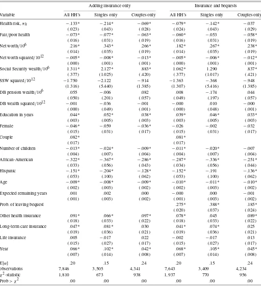
5.4.4 Tobits With Health Insurance and Bequests. As a fi-nal exercise, I reestimate the portfolio share tobit models after adding a set of indicator variables for various types of insur-ance against health-related expenditures, and then also adding the self-reported probability of leaving any bequests. Health in-surance, long-term care inin-surance, and life insurance all hedge against the direct financial risks associated with health shocks. Planned bequests may hedge informally through intergenera-tional care arrangements (Bernheim et al. 1985).
The first three columns in Table 6 show that additional health-related insurance is indeed associated with greater fi-nancial risk taking. Couples with additional health insurance beyond Medicare, for which everyone in the sample is age-eligible, have risky shares almost 10 percentage points higher
Table 5. Tobit regressions of portfolio shares using pooled AHEAD data with varying household composition, with household random effects or instrumental variables
Random effects Instrumental variables
Variable All HH’s Singles only Couples only All HH’s Singles only Couples only Health risk,πh −.112* −.179* −.064* −.449* −.664* −.283*
(.021) (.038) (.023) (.123) (.224) (.144)
Fair/poor health −.033* −.066* −.015 −.044 −.060 −.026
(.015) (.029) (.016) (.024) (.046) (.028)
Net worth/106 .197* .342* .186* .136* .258* .156*
(.014) (.032) (.019) (.017) (.042) (.025)
Net worth squared/1012 −.005* −.008* −.008* −.003* −.006* −.007*
(.000) (.001) (.001) (.001) (.001) (.002)
Social Security wealth/106 1.298* 1.833* .847 1.657* 1.986 1.418*
(.372) (.932) (.434) (.494) (1.374) (.545)
SSW squared/1012 −1.880 −1.311 −.706 −2.507 −3.059 −2.089
(1.200) (4.930) (1.316) (1.627) (7.156) (1.689)
DB pension wealth/106 .096* .136 .072 .056 −.287 .099
(.045) (.179) (.051) (.056) (.253) (.065)
DB wealth squared/1012 −.001* −.046 −.001 −.001 .043 −.001
(.000) (.043) (.000) (.001) (.057) (.001)
Education in years .041* .052* .028* .041* .046* .037*
(.003) (.005) (.003) (.004) (.007) (.004)
Female −.029* −.061 −.022 −.032 −.021 −.036
(.012) (.031) (.012) (.022) (.045) (.023)
Couple .087* .050*
(.020) (.024)
Number of children −.016* −.023* −.009 −.009 −.019 −.006
(.005) (.007) (.006) (.005) (.010) (.006)
African-American −.375* −.340* −.357* −.254* −.249* −.255*
(.042) (.053) (.047) (.048) (.077) (.064)
Hispanic −.206* −.208* −.255* −.168* −.176 −.180
(.058) (.099) (.067) (.076) (.132) (.094)
Age −.009* −.007* −.009* −.009* −.013* −.008*
(.002) (.003) (.002) (.002) (.005) (.003)
Expected remaining years .001 .001 .001 −.000 −.002 .001
(.001) (.002) (.001) (.002) (.004) (.002)
Year .061* .081* .046*
(.005) (.010) (.006)
E[α] .20 .15 .23 .23 .18 .27
Observations 8,172 3,668 4,504 3,267 1,467 1,800
χ2-statistic 1,006 559 465 602 228 318
Prob> χ2 .00 .00 .00 .00 .00 .00
Instrumented variable Health risk,πh
Number of instruments 5 5 5
First-stageF-stat 23.6 11.4 14.9
First-stageR2 .127 .130 .137
χ2-stat, overid 5.70 2.97 2.94
Prob> χ2, overid .223 .562 .414
NOTE: Standard errors are in parentheses. Asterisks denote significance at the 5% level. Data are pooled observations of individuals in the 1993 and 1995 AHEAD surveys, except for columns 4 and 5, which include only one wave each as a robustness check. The dependent variable isα, the risky portfolio share, constructed as described in the text and in the notes to Table 3. All regressions are tobits with limitsα=0 andα=1, and all include a constant term (not shown). Health risk,πh, is the self-assessed probability that medical expenses will
use up all household savings in the next five years, expressed as a fraction, 0 to 1. Health status may be reported as excellent, very good, good, fair, or poor. Net worth is total assets, including real estate, business, vehicular, and financial assets, minus debts. Social Security wealth and defined-benefit (DB) pension wealth are constructed as described in the text and in the notes to Table 3. Education is measured in years. Couple, African-American, and Hispanic are indicator variables. Kids is the number of surviving children. Remaining years are the expected number of remaining years before death as inferred from the individual’s subjective survivorship response. The fourth through sixth columns on the right side of the table report estimates from IV-tobit regressions where health risk is instrumented. The instrument set includes the lagged value of self-reported health risk, reports of mother’s age at death and father’s age at death, and two indicator variables for having ever smoked and whether smoking now. The use of lagged health risk restricts these IV-tobits to modeling portfolio choice in the 1995 wave only.
Table 6. Tobit regressions of portfolio shares using pooled AHEAD data with varying household composition and expanded insurance and bequest variables
Adding insurance only Insurance and bequests
Variable All HH’s Singles only Couples only All HH’s Singles only Couples only Health risk,πh −.133* −.214* −.069* −.079* −.142* −.037
(.023) (.043) (.028) (.024) (.043) (.029)
Fair/poor health −.073* −.077* −.063* −.060* −.053 −.058*
(.016) (.031) (.019) (.016) (.031) (.019)
Net worth/106 .216* .343* .266* .182* .267* .238*
(.014) (.035) (.019) (.014) (.035) (.019)
Net worth squared/1012 −.005* −.008* −.013* −.005* −.006* −.012*
(.000) (.001) (.001) (.000) (.001) (.001)
Social Security wealth/106 1.311* 2.127* .883* 1.062* 1.290 .837*
(.377) (1.025) (.420) (.377) (1.017) (.421)
SSW squared/1012 −1.750 −2.122 −.914 −1.363 −.368 −.948
(1.316) (5.440) (1.385) (1.307) (5.416) (1.385)
DB pension wealth/106 .055 −.006 .082 .008 −.174 .044
(.050) (.201) (.057) (.049) (.197) (.057)
DB wealth squared/1012 −.001 −.036 −.001 −.000 .010 −.000
(.000) (.049) (.001) (.000) (.048) (.001)
Education in years .044* .052* .038* .039* .046* .033*
(.003) (.005) (.003) (.003) (.005) (.003)
Female −.046* −.059 −.036* −.026 −.002 −.032
(.015) (.031) (.017) (.015) (.031) (.017)
Couple .082* .081*
(.017) (.017)
Number of children −.013* −.024* −.009* −.011* −.020* −.007
(.004) (.007) (.004) (.004) (.007) (.004)
African-American −.322* −.367* −.286* −.287* −.336* −.251*
(.033) (.056) (.043) (.034) (.056) (.044)
Hispanic −.151* −.204* −.128* −.152* −.191 −.136*
(.053) (.100) (.062) (.053) (.100) (.062)
Age −.009* −.008* −.009* −.010* −.011* −.010*
(.002) (.003) (.002) (.002) (.003) (.002)
Expected remaining years .001 .002 .000 −.000 .000 −.001
(.001) (.003) (.002) (.001) (.003) (.002)
Prob. of leaving bequest .275* .388* .185*
(.020) (.037) (.024)
Other health insurance .091* .066* .097* .078* .045 .089*
(.018) (.033) (.022) (.018) (.033) (.022)
Long-term care insurance .047* .081* .030 .041* .074* .025
(.019) (.036) (.021) (.019) (.036) (.021)
Life insurance .005 −.017 .022 −.002 −.017 .013
(.015) (.027) (.017) (.015) (.027) (.017)
Year .066* .102* .042* .068* .105* .045*
(.007) (.014) (.008) (.007) (.014) (.008)
E[α] .20 .15 .24 .20 .15 .24
observations 7,846 3,505 4,341 7,643 3,409 4,234
χ2-statistic 1,810 673 938 1,937 770 956
Prob> χ2 .00 .00 .00 .00 .00 .00
NOTE: Standard errors are in parentheses. Asterisks denote significance at the 5% level. Data are pooled observations of individuals in the 1993 and 1995 AHEAD surveys, except for columns 4 and 5, which include only one wave each as a robustness check. The dependent variable isα, the risky portfolio share, constructed as described in the text and in the notes to Table 3. All regressions are tobits with limitsα=0 andα=1, and all include a constant term (not shown). Health risk,πh, is the self-assessed probability that medical expenses will
use up all household savings in the next five years, expressed as a fraction, 0 to 1. Health status may be reported as excellent, very good, good, fair, or poor. Net worth is total assets, including real estate, business, vehicular, and financial assets, minus debts. Social Security wealth and defined-benefit (DB) pension wealth are constructed as described in the text and in the notes to Table 3. Education is measured in years. Couple, African-American, and Hispanic are indicator variables. Kids is the number of surviving children. Remaining years are the expected number of remaining years before death as inferred from the individual’s subjective survivorship response. The fourth through sixth columns on the right side of the table include the self-reported probability of leaving any bequest. All columns include indicator variables for having other health insurance beyond Medicare, for which all respondents are age-eligible, for having long-term care insurance, and for having life insurance.
than those who do not. Singles with such policies have 6.6 per-centage points more risk in their portfolios. Long-term care in-surance, that is, other than Medicaid, is significantly associated with greater financial risk taking for singles, but not for couples perhaps because it is partially redundant. Life insurance has no clear effect on risky portfolio shares, although the point esti-mate is at least positive for couples, the class of households for whom it should matter.
Including these insurance indicators does almost nothing to the health risk coefficients, as shown in the first row. That ad-ditional health insurance seems not to impact the size or the significance of the health risk variable is a telling result. If peo-ple feared risky health because of the specter of out-of-pocket medical expenditures sneaking through gaps in Medicare, then additional health insurance should decrease the association be-tween health risk and portfolio shares. But if health risk de-creases risk taking because the cross partial is negative, or be-cause shocks to health at older ages impede home production and raise the marginal utility of wealth, then additional medical expenditure insurance should have no effect, and this is what we find. A health insurance contract that simply paid out money in the poor health state could in principle lessen this exposure to the cross partial, but typical health insurance plans only cover a specific range of medical expenditures.
When I also include the self-reported probability of leaving any bequests as a covariate, I find results that are similar along one dimension and more revealing along another. The three rightmost columns in Table 6 show that portfolio shares for sin-gles and couples alike are positively associated with bequest motives and with additional insurance alike. Bequests have a stronger direct effect for singles, with an estimated coefficient of .388 versus .185 for couples. At the average effect of.275, an increase of 10 percentage points in the perceived chance of leaving any bequest is associated with an increase of almost 3 percentage points in the risky portfolio share. These results are consistent with intended bequests as wealth held in trust for younger generations with longer planning horizons and higher risk tolerance.
More striking is the impact of including bequests on the health risk coefficients: a drop in the magnitude of each by about one third. For couples, the inclusion of the bequest proba-bility renders health risk insignificant, but it remains significant among singles and the whole pooled sample. If intended be-quests are one side of a bargained informal care arrangement, these findings are consistent with a negative cross partial. Par-ents who fear debilitating health shocks because they require spending to replace home production may be able to hedge by securing future care from their children through promised in-heritances. This story is consistent with the larger IV-tobit co-efficients on health risk we found earlier; perceived health risk lowers the risky portfolio share but also incentivizes promised bequests, which raise the risky share.
6. DISCUSSION
Evaluating the links between health risk and portfolio selec-tion is a natural extension of two literatures: portfolio choice in the presence of background risk, and precautionary saving in response to health expenditure risk. Consistent with evidence
in the precautionary saving literature, this article finds that re-tired individuals perceive significant risks associated with fu-ture health shocks, and these perceptions are correlated with hedging behavior. I find that individuals over age 70 in the AHEAD hold safer financial portfolios when they view their future health as more risky. The riskiness of health tends to rise with age, so this result can partially explain the decline in finan-cial risk taking after retirement that we see in the data.
The precise motivation for decreasing exposure to financial risk when health is risky remains unclear, and there may be more than one. We know that there are significant gaps in cov-erage under Medicare and that out-of-pocket medical expendi-tures, though small on average, can also be catastrophic. When viewed as a type of background risk that raises the marginal utility of wealth by absorbing it, medical expenditure risk seems a likely candidate explanation.
But health shocks do more than absorb wealth. That addi-tional health insurance beyond Medicare does not reduce the association between health risk and portfolio shares in AHEAD data suggests a second and overlapping element is important: health-induced changes in the utility function. Theory suggests the sign of the cross partial derivative of utility over consump-tion and health should matter for portfolio choice. But depend-ing on their characteristics, health shocks could either raise, lower, or leave unchanged the enjoyment of consumption, and the empirical literature finds different signs at different ages and associated with different types of health shocks. When health shocks are disabling and thus hinder the ability of individuals to engage in essential activities and home production, the cross partial is negative, and sick individuals demand more funds to pay for lost home production. If health insurance simply paid money to the sick, then buying sufficient coverage could hedge this risk. But health insurance typically pays for specific goods and services and is not a direct cash transfer.
Patterns in the data are consistent with a negative cross partial for individuals. Household composition turns out to be impor-tant for the marginal association between risky portfolio shares and health risk. I find that the presence of a spouse hedges against risky future health, which suggests that individuals fear the loss of home production but expect a spouse to partially replace it. Owing to their closer proximity, spouses should be more direct hedges in this regard than children, and I find that they are. It is odd that the number of surviving children turns out to be negatively associated with financial risk taking in these data. Preferences over childbearing and risk are apparently neg-atively correlated, enough so that any hedging characteristics of simply having children are overwhelmed. But I find evidence that bequest motives hedge against health risk just like the pres-ence of a spouse. Strategic bequests planned in exchange for the promise of informal care would naturally offset the risk of a negative cross partial stemming from the potential loss of home production. If this story is true, the use of bequests as hedges against health risk can explain instrumental variables estimates that reveal larger direct effects of health risk on portfolio choice that are then moderated by intended bequests. Finally, I find that the presence of additional health insurance increases risk taking but does not reduce the marginal impact of risky health on port-folio shares. This is more consistent with individuals’ fear of an unhedged change in utility than of medical expenditures.