Deep Stock Representation Learning:
From Candlestick Charts to Investment Decisions
Guosheng Hu∗6Shanghai University of Finance and Economics 2
University of Shanghai for Science and Technology 3
Xiamen University 4
Independent Researcher 5
Queen Mary University of London 6Queen’s University Belfast 7The University of Edinburgh 8Yang’s Accounting Consultancy Ltd {huguosheng100, floodsung}@gmail.com,{hyx552211, yang kai 2008}@163.com, [email protected], [email protected]
[email protected], [email protected], [email protected], [email protected], [email protected]
Abstract
We propose a novel investment decision strategy based on deep learning. Many conventional algorithmic strategies are based on raw time-series analysis of historical prices. In con-trast many human traders make decisions based on visually observing candlestick charts of prices. Our key idea is to en-dow an algorithmic strategy with the ability to make decisions with a similar kind ofvisualcues used by human traders. To this end we apply Convolutional AutoEncoder (CAE) to learn an asset representation based on visual inspection of the as-set’s trading history. Based on this representation we propose a novel portfolio construction strategy by: (i) using the deep learned representation and modularity optimisation to cluster stocks and identify diverse sectors, (ii) picking stocks within each cluster according to their Sharpe ratio (Sharpe 1994). Overall this strategy provides low-risk high-return portfo-lios. We use the Financial Times Stock Exchange 100 Index (FTSE 100) data for evaluation. Results show our portfolio outperforms FTSE 100 index and many well known funds in terms of total return in 2000 trading days.
Introduction
Investment decision making is a classic research area in quantitative and behavioural finance. One of the most im-portant decision problems is portfolio construction and op-timisation (Markowitz 1952; Kelly 1956), which addresses selection and weighting of assets to be held in a portfolio. Financial institutions try to construct and optimise portfo-lios in order to maximise investor returns while minimising investor risk.
It is hard to predict the stock market due to partial in-formation and the involvement of irrational traders (Fama 1998) (who tend to over- or under-react on stock price (Barberis, Shleifer, and Vishny 1998)). Nevertheless, be-havioural finance argues the past price record impacts the market future performance (Balsara and Zheng 2006). Therefore many portfolio selection strategies are built on ‘judging and following’ historical data. Existing algorithmic methods to construct portfolios use raw time series data as input to drive optimisation via time-series analysis methods. However, human traders typically observe price history vi-sually, for example in the form of candlestick charts in order
∗These authors contributed equally to this work
to make trading decisions. Candlestick charts (Fig. 2) pro-vide a visual representation of four price parameters: lowest, highest, opening and closing price for the day. Thus current algorithmic strategies interpret the underlying data in a very different way than human traders due to the gap between raw time series and visual representations such as charts.
In this study we aim to endow an algorithmic portfolio op-timisation method with the ability to make decisions based on price history interpreted in a visual way more similar to human traders. In particular we develop a deep learn-ing (DL) approach to representlearn-ing price history visually and eventually driving portfolio construction. Convolutional DL approaches such as Convolutional AutoEncoder (CAE, unsupervised learning) (Masci et al. 2011) and Convolu-tional Neural Network (CNN, supervised learning) (LeCun et al. 1998), have achieved very impressive performance for analysing visual imagery. This has motivated researchers to adapt CNNs and CAEs to applications that are not naturally image-based. It is typically achieved by converting raw input signals from other modalities into images to be processed by CNNs or CAEs. Good results have been achieved for diverse applications in this way because of DL’s efficacy in captur-ing non-linearity, translation invariance, and spatial correla-tions. For example, traditional speech recognition methods used the 1-D signal vector, i.e. the raw input waveform, or its frequency domain projection (Rabiner and Juang 1993; Povey et al. 2011). In contrast an alternative approach is to convert the 1-D signal to a spectrogram, i.e. an image, in or-der to leverage the strength of CNNs to achieve promising recognition performance (Amodei et al. 2016). As another well known example, AlphaGo (Silver et al. 2016) repre-sents the board position as a 19×19 image, which is fed into a CNN for feature learning. With similar motivation, we ex-plore converting raw input data, (i.e., time-series) to images in order to leverage DL for better stock representation learn-ing, and hence ultimately better portfolio optimisation.
The first novelty of this study is exploiting deep learning to interpret price history data in a way more similar to hu-man traders by ‘seeing’ candlestick charts. To fully evaluate our approach, we further construct a complete portfolio gen-eration pipeline which requires a number of other elements. Our full investment strategy includes: (1) deep feature learn-ing by visual interpretation price history, (2) clusterlearn-ing the deep representation in order to provide a data-driven
mentation of the market, (3) actual portfolio construction.
For visual representation learning we take a 4-channel
stock time-series and synthesise candlestick charts to present price history as images. As we generate millions of train-ing images, we choose unsupervised CAE for representation learning, avoiding expensive big data labelling. The gen-erated charts are fed into a deep CAE to learn representa-tions which effectively encode the semantics of the historical time-series. In the nextclusteringstep, we aim to segment the market into diverse sectors in a data-driven way based on our generated visual representation. This is important to provide risk reduction by selecting a well diversified port-folio (Nanda, Mahanty, and Tiwari 2010; Tola et al. 2008). Popular clustering methods such as K-means are not suit-able here because they are non-deterministic and/or require a pre-defined numbers of clusters to find. In particular non-deterministic methods are not acceptable to real financial users. To address this we adapt the modularity optimization method (Newman 2006) – originally designed for network community structure – to stock clutsering. Specifically, we construct a network (graph) of stocks where each node cor-responds to a stock, and edges represent the correlation be-tween a pair of stocks (as represented by the learned visual feature vectors). To complete the pipeline we perform
port-folio constructionby the simple but effective approach of
choosing the best stock within each cluster according to their Sharpe ratio (Sharpe 1994). As we will see in our evaluation, this strategy provides a surprisingly approach to construct-ing portfolios that combine high returns with low-risk.
Our contributions can be summarised as follows:
• A novel deep learning approach that imitates human traders’ ability to ‘see’ candlestick charts. We convert raw 4-D stock time-series to candlestick images and use unsu-pervised convolutional autoencoders to learn a represen-tation for price history that encodes semantic information about the 4-D time series. To our knowledge, we are the first to apply deep learning techniques from computer vi-sion to investment decivi-sions.
• To support low-risk diversified portfolio construction, we segment the market by clustering stocks based on their learned deep features. To achieve deterministic cluster-ing without needcluster-ing to specify the number of clusters, we adapt modularity optimisation, originally used for detect-ing community structure in networks, to stock clusterdetect-ing.
• We evaluate our strategy using Financial Times Stock Ex-change 100 Index (FTSE 100) stock data. Results show (a) our learned deep stock representation effectively cap-tures semantic information. (b) our portfolio construction strategy outperforms the FTSE 100 index and many well-known funds including 2 big funds (CCA, VXX) and the 3 best performed funds (IEO, PXE, PXI) recommended by Yahoo in terms of total return in 2000 trading days, showing the effectiveness of our investment strategy.
Related Work
Investment Decision Strategy Portfolio optimisation is a mainstay of investment decision making. There are two
mainstream directions of investigating the optimal allocation of capital with different perspectives on period selection: (i) The Mean Variance Theory (Markowitz 1952; Markowitz 1959; Markowitz and Todd 2000) chooses a single-period and optimises the portfolio by the trading-off of the ex-pected return and the variance of return. Derived from this strategy, many well-known ratios were proposed as objec-tive functions to drive portfolio optimisation. For example the Sharpe ratio (Sharpe 1994) and Omega ratio (Keating and Shadwick 2002). In other words, the mean variance the-ory directs investment based on the ‘risk-return’ profile of a portfolio. (ii) The Capital Growth Theory (Kelly 1956; Hakansson and Ziemba 1995) defines the optimal strategy in dynamic and reinvestment situations and primarily focuses on the growth rate. Unlike mean variance theory, capital growth pays great attention to time dependence. It analyses the information of different time series, such as asset trees (Onnela et al. 2003), which uses time dependence to con-struct a tree based on the best classification of stocks. Our strategy combines the ideas of (i) and (ii) by using Sharpe ratio and encoding time dependence with deep learning.
...
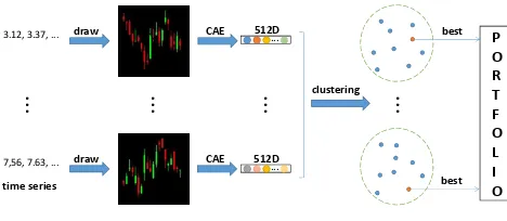
Figure 1: Schematic illustration of our investment decision pipeline. The architecture of CAE is detailed in Fig. 3.
Methodology
Our overall investment decision pipeline includes three main modules: deep feature learning, clustering, and portfolio construction. Fordeep feature learning, raw 4-channel time series data describing stock price history are converted to standard candlestick charts. These charts are then fed into a deep CAEs for visual feature learning. These learned fea-tures provide a vector embedding of a historical time-series that captures key quantitative and semantic information. Next weclusterthe features in order to provide a data-driven segmentation of the market to underpin subsequent selection of a diverse portfolio. Many common clustering methods are not suitable here because they are non-deterministic or re-quire predefinition of the number of clusters. Thus we adapt modularity optimisation for this purpose. Finally, we per-formportfolio constructionby choosing stocks with the best performance measured by Sharpe ratio (Sharpe 1994) from each cluster. The overall pipeline is summarised schemati-cally in Fig. 1. Each component is discussed in more detail in the following sections.
Autoencoders
An AutoEncoder (AE) is a typical artificial neural network for unsupervised feature learning. It learns an effective rep-resentation without requiring data labels, by encoding and reconstructing the input via bottleneck. An AE consists of an encoder and a decoder: The encoder uses raw data as in-put and produces representation as outin-put and the decoder uses the learned feature from the encoder as input and re-constructs the original input as output.
For simplicity, we describe formally only a fully-connected AE with 3 layers: encoding, hidden and decoding layer. The encoderfprojects the inputxto the hidden layer representation (encoding)h. Typically,f includes a linear transform followed by a nonlinear one:
h=f(x) =σ(Wx+b) (1) whereW is the linear transform andbis the bias.σis the nonlinear (activation) function. There are many ‘activation’ functions available such as sigmoid, tanh and RELU. We use RELU (REctified Linear Units) in this work.
The decodergmaps the hidden representationhback to the inputx via another linear transformW′ and the same
‘activation’ functionσas shown in Eq. (2):
x=g(h) =σ(W′h+b′) (2)
Figure 2: Stock candlestick chart. (a) Candlestick explana-tion (b) One sample chart from stock ‘Royal Dutch Shell Plc Class A’ between 03/01/2017 and 31/01/2017.
To optimise {W′, W,b,b′}, the AE uses the cost
func-wherexirepresents theith one ofNtraining samples. Using
the objective in Eq. (3) the AE parameters can be learned via mini-batch stochastic gradient descent.
Convolutional Autoencoders Traditional AEs ig-nore the 2D image structure. Convolution AutoEncoders (CAEs) (Masci et al. 2011) extend vanilla AEs with convo-lution layers that help to capture the spatial information in images and reduce parameter redundancy compared to AEs. We use convolutional autoencoders in this work to process stock charts visually.
Deep Feature Learning with Convolutional
Autoencoders
Chart Encoding To realise an algorithmic portfolio con-struction method based on visual interpretation of stock charts, we need to convert raw price history data to an image representation. Our raw data for each stock is a 4-channel time series (the lowest, the highest, open, and closing price for the day) in a 20-day time sequence. We use computer graphics techniques to convert these to a candlestick chart represented as a RGB image as shown in Fig. 2. The whisker plots describe the four raw channels, with color coding de-scribing whether the stock closed higher (green) or lower (red) than opening. An encoded candlestick chart image pro-vides the visual representation of one stock over a 20-day window for subsequent visual interpretation by our deep learning method.
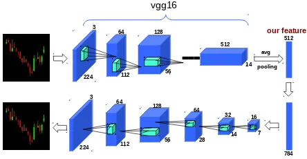
vgg16
Figure 3: Overview of our CAE architecture. We follow the encoder (top) - decoder (bottom) framework. The 512D fea-ture following average pooling provides our representation for clustering and portfolio construction.
fully connected with the 512D embedding layer. Following 6 upsampling deconvolution layers eventually reconstruct the input based on our 512D feature. When trained with a re-construction objective, the CAE network learns to compress input images to the 512D bottleneck in a manner that pre-serves as much information as possible in order to be able to reconstruct the input. Thus this single 512D vector encodes the 20-day 4-channel price history of the stock, and will pro-vide the representation for further processing (clustering and portfolio construction).
Clustering
We next aim to provide a mechanism for diversified – and hence low risk – portfolio selection. Unlike some existing methods which calculate the stock correlation based on the raw time series, in this paper, we use our learned features in a clustering step in order to segment the market. As dis-cussed before many existing clustering methods are non-deterministic or require pre-specification of the number of clusters, which make them unsuited for our application do-main. To solve these problems, we introduce the network modularity method to find the cluster structure of the stocks, where each stock is set as one node and the link between each pair of stocks is set as the correlation calculated by the learned features (Blondel et al. 2008). Modularity is the frac-tion of the links that fall within the given group minus the expected fraction if links are distributed at random. Mod-ularity optimisation is often used for detecting community structure in networks. It operates on a graph (of stocks in our case), and updates the graph to group stocks so as to eventu-ally achieve maximum modularity before terminating. Thus it does not need a specified number of clusters and is not affected by initial node selection, which
Algorithm Description One 20-day history of the entire market is represented as a single graph. Each stock corre-sponds a single node in the initial graph, and is represented by our CAE learned feature. The cosine similarity between these features is then used to weight the edges of the graph connecting each stock according to their similarity.
The Blondel method (Blondel et al. 2008) for cluster
de-tection provides a fast greedy approach based on modularity optimisation (Newman 2006). It can be divided into two it-erative steps:
1. Initially, each node in network is considered a cluster. Then, for each nodei, one considers its neighbourjand calculates the modularity increment by movingifrom its cluster to the cluster ofj. The nodeiis placed in the clus-ter where this increment is maximum, but only if this in-crement is positive. If no positive inin-crement is possible, the nodeistays in its original cluster. This process is ap-plied repeatedly for all nodes until no further increment can be achieved.
2. The second step is to build a new network whose nodes are the clusters found in the first step. The weights of the links between the new nodes are given by the sum of the number of the links between nodes from the correspond-ing component clusters now included in that node. The key notion of modularity increment∆Q(x, y), wherex
is one of the new nodes andyisx’s neighbour, is defined as:
∆Q(x, y) = [ein,cy+ 2kx,cy
number of the links inside clustercy andetot,cy denotes the
sum of degrees of nodes in the clustercy,kx is the degree
of the nodex,kx,cy is the sum of the links from the nodex
to the nodes in the clustercyandmis the number of all the
links in the network.
The end result is a segmentation of the market into a max-imum modularity graph withKnodes/clusters, where each node contains all the stocks that cluster together. It should be noticed that whether the graph is fully connected or not, the Blondel method finds a hierarchical cluster structure.
Portfolio Construction and Backtesting
So far we have described the parts of our strategy designed to maintain low risk via high diversity (stock clustering driven by learned deep features). Given the learned stock clustering (market segmentation) , we finally describe how a complete portfolio is constructed by picking diverse yet high-return stocks, as well as our portfolio evaluation process.
Stock Performance Return (profit on an investment) is defined asrt = (Vf−Vi)/Vi, whereVf andVi are the
fi-nal and initial values, respectively. For example, to compute daily stock return,VfandViare closing prices of today and
yesterday, respectively. We measure the performance of one particular stock over a period using the Sharpe ratio (Sharpe 1994) s = r/σr, where r is the mean return, σr is the
standard deviation over that period. Thus the Sharpe ratios
encodes a tradeoff of return and stability. Maximum Draw-down (MDD) is the measure of decline from peak during a specific period of investment: MDD= (Vt−Vp)/Vp, where VtandVpmean the trough and peak values, respectively.
the highest Sharpe ratio (Sharpe 1994) within each cluster. We then hold the selected portfolio for 10 days. Over these following 10 days, we evaluate the portfolio by computing our ‘compound return’ for each selected stock. The over-all return of one portfolio in in these 10 days is the average compound return of all the selected stocks. The stride for the 20-day window is 10 in this work.
The process of portfolio selection/optimisation in Finance is analogous to the process of training in machine learning, and the subsequent return computation is analogous to the testing process.
Since the modular-optimisation based clustering discov-ers the number of stocks in a data driven way, in differ-ent trading periods we may have differdiffer-ent number of clus-ters. Assume that we obtainK1 clusters in one period and
will selectK2 stocks to construct one portfolio. Then, let-tingQandR indicate quotient and remainder respectively in[Q, R] = K2/K1:K2 stocks are picked by taking (i)Q
stocks from each of theK1clusters and (ii) the remainingR
best performing stocks across allK1clusters. Then, we allo-cate equally1/K2of the fund to each of the chosen stocks.
Experiments
We first introduce our dataset and experimental settings. Then we analyse the outputs of feature learning and cluster-ing. Finally, we compare our investment strategy (feature ex-traction, clustering, portfolio optimisation) as a whole with other strategies.
Dataset and Settings
Preprocessing For evaluation, we use the stock data of Fi-nancial Times Stock Exchange 100 Index (FTSE 100). The FTSE 100 is a share index of the 100 companies listed on the London Stock Exchange with the highest market capitalisa-tion. It effectively represents the economic conditions of the UK and even the EU. We use all the stocks in FTSE 100 from 4th Jan 2000 to 14th May 2017. We use the adjusted stock price (accounting for stock splits, dividends and dis-tributions). Every 20-day 4-channel (the lowest price of the day, the highest price, open price, closing price) time series generates a standard candlestick chart. We generate 400K FTSE100 charts in all. The training images for our CAE are candlestick charts rendered as 224×224 images to suit our VGG16 architecture (Simonyan and Zisserman 2014).
Implementation Details The batch size is 64, learning rate is set to 0.001, and the learning rate decreases with a factor of 0.1 once the network converges.
Qualitative Results
Visualising and Understanding Deep Features First, we visualise the input and reconstructed candlestick charts in Fig. 4. We can see that the reconstructed charts effectively capture the variations of the inputs showing the efficacy of our CAE for unsupervised learning and the representational capacity of our 512D feature (CAE bottleneck layer). Note that as is commonly the case for autoencoders, the back-ground is slightly grey because the pixel values of recon-structed background are close to 0, but not equal to 0.
Figure 4: Candlestick charts as input (top) and reconstructed (bottom) by our CAE.
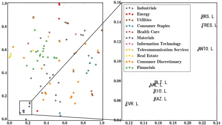
Figure 5: t-SNE visualisation of FTSE 100 CAE features. One color indicates one industrial sector. The stocks on the right are all from Sector Materials: RRS.L (Randgold Resources Limited), FRES.L (Fresnillo PLC), ANTO.L (Antofagasta PLC), BLT.L (BHP Billiton Ltd), AAL.L (An-glo American PLC), RIO.L (Rio Tinto Group), KAZ.L (KAZ Minerals), EVR.L (EVRAZ PLC)
Second, we visualise the learned features. The features of one whole year (2012) for one particular stock are con-catenated to form a new feature. These new features of all the stocks are visualised in Fig. 5 using the t-Distributed Stochastic Neighbor Embedding (t-SNE) (Maaten and Hin-ton 2008) method. One color indicates one industrial sec-tor defined by bloomberg (https://www.bloomberg. com/quote/UKX:IND/members). From Fig. 5, we can see the stocks with similar semantics (industrial sector) are represented close to each other in the learned feature space. For example, Materials related stocks are clustered. This il-lustrates the efficacy of our CAE and learned feature for cap-turing semantic information about stocks.
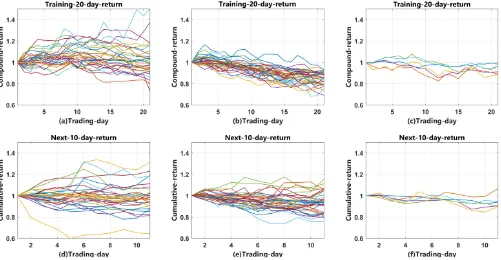
Figure 6: Visualisation of modularity optimisation clustering results. Row 1: compound returns of all the stocks in 3 clusters during portfolio optimisation (20 trading days), Row 2: compound returns during test (in the following 10 trading days).
example the top-left cluster represents a position of no net profit or loss, but high fluctuation. The top-middle cluster represents stocks with a characteristic of continuous steep decline; while the top-right cluster represents those with continuous slight decline. Clearly the segmentation method has allocated stocks to clusters with distinct trajectory char-acteristics. During testing the three corresponding clusters on the bottom behave quite similarly as those above. This demonstrates the momentum effect (Jegadeesh and Titman 1993), and the consistency between portfolio selection (20-day, training) and return computation (10-(20-day, testing).
Quantitative Results
For quantitative evaluations, we apply 7 measures for evalu-ation: Total return, daily Sharpe ratio, max drawdown, daily mean return, monthly mean return, yearly mean return, and win year. Win year indicates the percent of the winning years. The other measures are defined in the section of ‘Port-folio Construction and Backtesting’. We choose K2 = 5
stocks to construct all the portfolios compared.
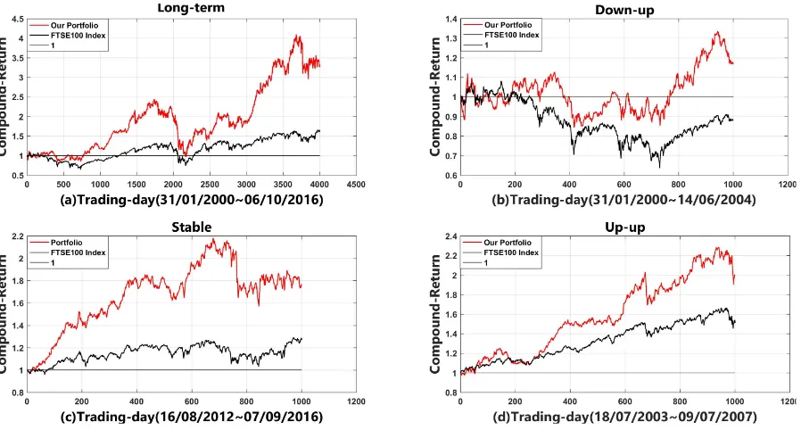
Comparison with FTSE 100 Index We perform back-testing to compare our full portfolio optimisation strategy against the market benchmark (FTSE 100 Index). In Fig. 7, we compare with FTSE 100 index. Fig. 7 (a) shows the com-parison over a long-term trading period (4K trading days, 31/01/2000 - 06/10/2016) showing the overall effectiveness of our strategy. Note that it is very difficult for funds to con-sistently outperform the market index over an extended pe-riod of time due to the complexity and diversity of market
variations. In Fig. 7 (b)-(c) we show specific shorter term periods where the market is behaving very differently in-cluding down-up (b), flat (c) and bullish (d). The overall dynamic trends of our strategy reflect the conditions of the market (meaning that the stocks selected by our strategy are representative of the market), yet we outperform the market even across a diverse range of conditions (b-c), and over a long time-period (a).
Feature and Clustering
Figure 7: Our portfolio vs FTSE 100 Index
Table 1: Comparison with well-known Funds
CCA VXX IEO PXE PXI Ours
Total Return (↑) 117.0% -99.9% 89.9% 101.6% 152.2% 215.4%
Daily Sharpe (↑) 0.7 -1.1 0.4 0.4 0.6 0.8
Max Drawdown (↑) -22.2% -99.9% -56.8% -57.6% -59.3% -30.9% Daily Mean Return (↑) 10.9% -67.7% 12.7% 13.4% 15.9% 16.7%
Monthly Mean Return (↑) 10.7% -66.4% 11.5% 12.4% 14.9% 16.6%
Yearly Mean Return (↑) 6.5% -44.6% 5.0% 8.2% 9.4% 11.8%
Win Years (↑) 62.5% 0.0% 62.5% 50.0% 75.0% 62.5%
Table 2: Comparison of Features and Clustering Methods.
R-M D-M (Ours) D-K
Total Return (↑) 208.8% 283.5% 272.6% Daily Sharpe (↑) 0.44 0.50 0.49 Max Drawdown (↑) -55.6% -60.5% -59.0 % Daily Mean Return (↑) 9.7 % 11.1% 10.9% Monthly Mean Return (↑) 8.7% 10.0% 9.9%
Yearly Mean Return (↑) 9.6% 10.0 % 11.19% Win Years (↑) 64.71% 69.52% 66.31%
Comparison with Funds To further analyse the effective-ness of our strategy, we compare our strategy with well known public funds in stock market. Specifically, we se-lect 2 big funds (CCA and VXX) and the top 3 best per-formed funds (IEO, PXE, PXI) recommended by YAHOO ( https://finance.yahoo.com/etfs). Note that the ranking of funds change over time. The fund data is obtained from Yahoo Finance. Because VXX starts from 20/01/2009, this evaluation is computed over 2K trading days (20/01/2009-09/01/2017). From Table 1, our port-folio achieved the highest returns: Total (215.4%), daily
(16.7%), monthly (16.6%), yearly (11.8%) in 2000 trading days, showing the strong profitability of our strategy. We also achieved the highest daily Sharpe ratio (0.8), meaning that we effectively balance the profitability and variance. We achieve the 2nd lowest max drawdown, meaning that our method can effectively manage the investment risk. In most years (62.5%), our portfolio makes a profit. It is only slightly worse than PXI in terms of 75.0% of profitable years. This shows the stability of our strategy.
Conclusions
References
[Amodei et al. 2016] Amodei, D.; Ananthanarayanan, S.; Anubhai, R.; et al. 2016. Deep speech 2: End-to-end speech recognition in english and mandarin. InICML, 173–182. [Balsara and Zheng 2006] Balsara, N., and Zheng, L. 2006.
Profiting from past winners and losers. Journal of Asset
Management.
[Barberis, Shleifer, and Vishny 1998] Barberis, N.; Shleifer, A.; and Vishny, R. 1998. A model of investor sentiment.
Journal of financial economics.
[Blondel et al. 2008] Blondel, V. D.; Guillaume, J.-L.; Lam-biotte, R.; and Lefebvre, E. 2008. Fast unfolding of com-munities in large networks.Journal of statistical mechanics: theory and experiment.
[Fama 1998] Fama, E. F. 1998. Market efficiency, long-term returns, and behavioral finance. Journal of financial eco-nomics.
[Hakansson and Ziemba 1995] Hakansson, N. H., and Ziemba, W. T. 1995. Capital growth theory. Handbooks in
Operations Research and Management Science9:65–86.
[He et al. 2016] He, K.; Zhang, X.; Ren, S.; and Sun, J. 2016. Deep residual learning for image recognition. InCVPR. [Huang et al. 2016] Huang, G.; Liu, Z.; Weinberger, K. Q.;
and van der Maaten, L. 2016. Densely connected convolu-tional networks. arXiv preprint arXiv:1608.06993.
[Jegadeesh and Titman 1993] Jegadeesh, N., and Titman, S. 1993. Returns to buying winners and selling losers: Impli-cations for stock market efficiency. The Journal of finance
48(1):65–91.
[Keating and Shadwick 2002] Keating, C., and Shadwick, W. F. 2002. A universal performance measure. Journal
of performance measurement.
[Kelly 1956] Kelly, J. L. 1956. A new interpretation of in-formation rate.Bell Labs Technical Journal.
[Kingma and Welling 2013] Kingma, D. P., and Welling, M. 2013. Auto-encoding variational bayes. arXiv preprint
arXiv:1312.6114.
[Krizhevsky, Sutskever, and Hinton 2012] Krizhevsky, A.; Sutskever, I.; and Hinton, G. E. 2012. Imagenet classifi-cation with deep convolutional neural networks. InNIPS, 1097–1105.
[LeCun et al. 1998] LeCun, Y.; Bottou, L.; Bengio, Y.; and Haffner, P. 1998. Gradient-based learning applied to docu-ment recognition. Proceedings of the IEEE.
[Lee et al. 2009a] Lee, H.; Grosse, R.; Ranganath, R.; and Ng, A. Y. 2009a. Convolutional deep belief networks for scalable unsupervised learning of hierarchical representa-tions. InICML. ACM.
[Lee et al. 2009b] Lee, H.; Pham, P.; Largman, Y.; and Ng, A. Y. 2009b. Unsupervised feature learning for audio classi-fication using convolutional deep belief networks. InNIPS, 1096–1104.
[Lowe 1999] Lowe, D. G. 1999. Object recognition from local scale-invariant features. InICCV. IEEE.
[Maaten and Hinton 2008] Maaten, L. v. d., and Hinton, G. 2008. Visualizing data using t-sne. Journal of Machine
Learning Research2579–2605.
[Markowitz and Todd 2000] Markowitz, H. M., and Todd, G. P. 2000. Mean-variance analysis in portfolio choice and capital markets, volume 66. John Wiley & Sons.
[Markowitz 1952] Markowitz, H. 1952. Portfolio selection.
The journal of finance.
[Markowitz 1959] Markowitz, H. 1959. Portfolio selection: Efficient diversification of investments. cowles foundation monograph no. 16.
[Masci et al. 2011] Masci, J.; Meier, U.; Cires¸an, D.; and Schmidhuber, J. 2011. Stacked convolutional auto-encoders for hierarchical feature extraction. Artificial Neural
Net-works and Machine Learning–ICANN 201152–59.
[Nanda, Mahanty, and Tiwari 2010] Nanda, S.; Mahanty, B.; and Tiwari, M. 2010. Clustering indian stock market data for portfolio management. Expert Systems with Applications. [Newman 2006] Newman, M. E. 2006. Modularity and
com-munity structure in networks. Proceedings of the national academy of sciences.
[Onnela et al. 2003] Onnela, J.-P.; Chakraborti, A.; Kaski, K.; Kertesz, J.; and Kanto, A. 2003. Dynamics of mar-ket correlations: Taxonomy and portfolio analysis. Physical Review E.
[Perronnin, S´anchez, and Mensink 2010] Perronnin, F.; S´anchez, J.; and Mensink, T. 2010. Improving the fisher kernel for large-scale image classification. ECCV 2010
143–156.
[Povey et al. 2011] Povey, D.; Ghoshal, A.; Boulianne, G.; Burget, L.; Glembek, O.; Goel, N.; Hannemann, M.; Motlicek, P.; Qian, Y.; Schwarz, P.; et al. 2011. The kaldi speech recognition toolkit. InIEEE 2011 workshop on
auto-matic speech recognition and understanding, number
EPFL-CONF-192584. IEEE Signal Processing Society.
[Rabiner and Juang 1993] Rabiner, L. R., and Juang, B.-H. 1993. Fundamentals of speech recognition.
[Sharpe 1994] Sharpe, W. F. 1994. The sharpe ratio. The
journal of portfolio management.
[Silver et al. 2016] Silver, D.; Huang, A.; Maddison, C. J.; Guez, A.; Sifre, L.; Van Den Driessche, G.; Schrittwieser, J.; Antonoglou, I.; Panneershelvam, V.; Lanctot, M.; et al. 2016. Mastering the game of go with deep neural networks and tree search. Nature.
[Simonyan and Zisserman 2014] Simonyan, K., and Zisser-man, A. 2014. Very deep convolutional networks for large-scale image recognition.arXiv preprint arXiv:1409.1556. [Szegedy et al. 2015] Szegedy, C.; Liu, W.; Jia, Y.; Sermanet,
P.; Reed, S.; Anguelov, D.; Erhan, D.; Vanhoucke, V.; and Rabinovich, A. 2015. Going deeper with convolutions. In
CVPR.