T H E J O U R N A L O F H U M A N R E S O U R C E S • 45 • 2
Evidence from Displacement-Driven Income
Shocks
Jason M. Lindo
A B S T R A C T
This paper explores the causal link between income and fertility by analyz-ing women’s fertility response to the large and permanent income shock generated by a husband’s job displacement. I find that the shock reduces total fertility, suggesting that the causal effect of income on fertility is positive. A model that incorporates the time cost of children and assorta-tive matching of spouses can simultaneously explain this result and the negative cross-sectional relationship. I also find that a husband’s displace-ment accelerates childbearing, which is consistent with lifecycle models of fertility in which the incentive to delay is driven by expected earnings growth.
I. Introduction
Are children inferior goods? Economists have long wrestled with this question because cross-sectional evidence suggests that family size and income are negatively correlated: high income families tend to have few children and, analo-gously, high income countries tend to have low fertility rates. Further, time-series data frequently show that developing countries transition towards lower fertility rates as they industrialize. The negative relationship between income and fertility is not itself inconsistent with standard consumer choice models of household fertility. However, within that theoretical framework, it is inconsistent with the presumption that children are normal goods. Seminal papers by Becker (1960), Becker and Lewis (1973), and Willis (1973) reconcile this apparent conflict with economic theory by
Jason M. Lindo is an assistant professor of economics at the University of Oregon. He is especially grateful to his dissertation chairs, Marianne Page and Ann Huff Stevens, for their guidance and sup-port. He also thanks Colin Cameron, Greg Clark, Hilary Hoynes, Doug Miller, participants at the Uni-versity of California, Davis brownbag series, participants at the 2008 WEAI Conference, and two anon-ymous referees for their helpful suggestions. The data used in this article can be obtained beginning October 2010 through September 2013 from Jason Lindo, Department of Economics, University of Oregon, jlindo@uoregon.edu.
[Submitted February 2008; accepted November 2008]
developing household models in which both child quantity and quality enter the household utility function and budget constraint. Others have tried to solve the puz-zle with models that incorporate the time costs of children. These models, however, tend to be based on the assumption that the observed relationship between income and fertility is causal. In fact, little is known about what underlies this correlation.1
This paper begins to fill this important gap in the literature by analyzing the fertility impact of the large and permanent income shock generated by a husband’s job displacement.
This paper also aims to improve our understanding of the timing of fertility by estimating women’s dynamic fertility response to the shock. Many theoretical mod-els analyze fertility in a lifecycle framework because it provides another dimension along which households can adjust fertility in response to economic incentives. A household not only chooses how many children to have, but also when to have them. In these theoretical models, a credit-constrained household spaces out its children to balance the desire to have children early (so that the benefits can be enjoyed for more periods) with the desire to have children later when the husband’s earnings are higher. Thus, these models predict that a flatter earnings trajectory will lead to accelerated fertility.2 Analyzing the dynamic fertility response to a husband’s job
displacement, which typically has a permanent effect on earnings growth, provides a unique opportunity to test this prediction.
Across the world, influential fertility policies have been put into place based on the assumed relationship between fertility and economic well-being. In some devel-oping countries, overpopulation is considered to be such a serious impediment to economic growth that laws restrict the number of children couples are allowed to have. China’s one child per family policy highlights this end of the spectrum.3Such
laws are motivated by the belief that reducing population is a crucial step towards joining the rest of the world in prosperity. However, the efficacy of such policies is the source of much controversy—in part because little is known about the causal relationship between fertility and income.
On the other hand, with nearly one hundred countries below their replacement rates, there are many places where low fertility rates are of concern.4While cultural
factors are sometimes involved, the anxiety is usually driven by the idea that low fertility will result in an aging population in which support of the elderly places an undue burden on young workers. In response, many governments have implemented policies providing financial incentives for having children. Quebec, Canada led the way in 1988 by providing a “baby bonus” which paid up to nearly $6,000 to families having a child. Despite the high costs of such programs, many countries have fol-lowed suit including Singapore (2001), Australia (2004), Italy (2005), and Poland (2006). Ulyanovsk, Russia has implemented what is perhaps the most original pro-natalist policy, declaring September 12 the “Day of Conception.” In addition to
1. Becker (1960) argues that knowledge about birth control might be a factor. 2. See Heckman and Willis (1975), Wolpin (1984), and Newman (1988).
3. Similarly in India, while there are no nationwide restrictions, some states have a two child per family policy for members of village councils and civil servants.
getting the day off work, couples who “give birth to a patriot” nine months later on Russia’s Independence Day win prizes such as money, cars, and refrigerators (Stro-mova 2007).
Whether the concern is about high fertility rates or low fertility rates, it is im-portant to understand how income can influence fertility both directly and indirectly. The results of this paper can be helpful in evaluating the consequences of policy interventions that alter family income. In the United States, for example, one of the main concerns with welfare policies is that families might use the additional income to have more children. The empirical evidence on this issue is mixed.5
Most studies that analyze the relationship between income and fertility make a weak case, if any, that their measure of income is exogenous with respect to their measure of fertility even though there are at least two reasons this is unlikely to be true. First, reverse causality is possible. For example, parents may adjust the amount they work or the amount they invest in human capital based on the number of children they plan to have.6Second, there are likely to be unobservables that drive
both income and fertility. For example, individuals with high discount rates may have low incomes and more unplanned children.
The ideal way to estimate the causal impact of family income on fertility would be via an experiment that randomly assigned individuals different levels of perma-nent income. The next best alternative might randomly add to or take away from couples’ incomes. While such experiments are unlikely to ever be conducted, this paper is motivated by the idea that husbands’ job displacements present a natural experiment of this type.7 It is well established that job losses result in large and
permanent losses in earnings—the permanent nature of the shock has been docu-mented using the same data set used in this study, the Panel Survey of Income Dynamics (as well as many other data sets).8 Prior studies have also shown that
workers who will be displaced in the following year have low subjective probabilities
5. In separate reviews of the literature, Hoynes (1997) concludes that the effects are often insignificant or small in magnitude, while Moffitt (1998) concludes that welfare likely does impact fertility (although he explains that his conclusion is weakened by the lack of robustness).
6. Angrist and Evans (1998) provide the best evidence against this concern for husbands. Using the sex composition of the first two children as an instrument for having more than two children, they do not find a statistically significant impact on fathers’ earnings or employment. However, their estimates must be interpreted with caution as they only analyze the effect of having more than two children versus two children.
7. After the completion of an earlier draft of this paper, I discovered another work-in-progress (Amialchuk 2006) exploring the impact of husbands’ job losses on fertility. My paper differs from this paper, which finds delays in first and second births, in a number of important aspects. While Amialchuk (2006) uses a hazard model, I use a generalized difference-in-difference approach that allows me to control for fixed unobservable characteristics related to both fertility and the probability of having a displaced husband. I also do the analysis at the woman level rather than the couple level so that I can capture fertility effects that may be driven by marital separations following a job loss. I also omit women who were married prior to 1968 to reduce the probability that a husband’s first displacement is missed.
of job loss, which lends confidence to the notion that displacements are largely unanticipated.9
The main advantage of my research design is the transparent and plausibly ex-ogenous source of variation in husbands’ earnings. Like Jacobson, LaLonde, and Sullivan (1993) and Stevens (1997), I employ an individual fixed effects model to estimate the impact of a displacement so that the estimates will be unbiased even if there are fixed unobservable characteristics related to both displacements and the outcome of interest. In addition, I confirm that the results are robust to using a displaced sample that is limited to women whose husbands lost their jobs due to plant or business closures, since these types of displacements are more likely to be exogenous than the broader category which includes displacements resulting from husbands being laid off or fired.
Another important advantage of my research design is that the magnitude of the shock generated by a husband’s job displacement is large. Generally, the income elasticity that has been implied by cross-sectional estimates is small. As a result, a large shock like that resulting from a husband’s job displacement might be necessary to identify an effect.
I find that a shock to husbands’ earnings impacts both short and long-run fertility. Consistent with dynamic models of fertility, I find that the shock accelerates the timing of fertility. Women are significantly more likely to have children in the years immediately following a husband’s job displacement but significantly less likely to have children many years later. The immediate increase in fertility is outweighed by the subsequent decline, resulting in a net reduction in the number of children. This implies that the causal relationship between husbands’ earnings and total fertility is positive.
While the most salient feature of a husband’s displacement is clearly the large reduction in his earnings, an important caveat to my findings is that the estimated impact of a husband’s job loss on fertility might be generated by aspects of the shock other than the loss of income. For example, a husband’s job loss may impact fertility because of an impact on stress or women’s work activity that is unrelated to the impact on income. However, researchers using panel data to study the impacts of unemployment on mental health have not found significant effects.10And while
it has been shown that husbands’ displacements cause women to work more (Ste-phens 2002), it is reasonable to think that this effect is mostly driven by the desire to compensate for his lost earnings. Finally, while Charles and Stephens (2004) find that being laid off or fired increases the probability of divorce but that a job loss due to a plant or business closure does not affect divorce, I find evidence that both types of displacements lead to the fertility response described above. This indicates that the estimated response is not driven by displacements impact on marital dis-solutions.
The remainder of this paper is organized as follows. Section II discusses house-hold models of fertility. Section III reviews some of the related empirical literature.
9. Manski and Straub (2000) find a median subjective probability of 5 percent while Stephens (2004) finds a median of 20 percent.
Section IV describes the data while Section V describes the empirical methodology. Section VI presents the main results. Section VII discusses the results in detail and Section VIII concludes.
II. Theoretical Considerations
In general, economists have used static models of the household to examine the determinants of completed fertility and dynamic models to examine the determinants of the timing of fertility. The following discussion, which focuses on the role of husbands’ earnings in these models, is also separated along these lines. It draws from Becker (1991), Hotz, Klerman, and Willis (1997), and Jones, Schoon-broodt, and Tertilt (2008).
A. Static Models of the Household Fertility Decision
In a basic static model of the household, the relationship between income and child quantity can be thought of like the relationship between income and any other good. Thus, in such a model, the frequently observed negative relationship between income and fertility suggests that child quantity is an inferior good (assuming that the re-lationship is causal). Beginning with Becker’s (1960) seminal work introducing the concept of child quality, theorists have expended a great deal of effort trying to reconcile the empirical relationship with the notion that children ought to be a normal good.
Becker and Lewis (1973) and Willis (1973) explain that the negative relationship can be generated by incorporating the interaction between child quantity and child quality into the household budget constraint. This interaction term captures the costs of child quality that must be spent on each child individually, such as college tuition. In this model, increasing either quantity or quality increases the shadow cost of the other. For example, sending children to college rather than high school makes ad-ditional children more expensive. Similarly, having an adad-ditional child makes it relatively expensive to send the children to college. The effects of income are not straightforward in this type of model because, through the direct impact on child quantity and child quality, income effects induce price effects. Consider a reduction in income under the assumptions that both child quantity and child quality are normal goods although the income elasticity is greater for quality than for quantity. Initially, the income loss will cause a “pure income effect” (holding shadow prices constant) that reduces both quantity and quality. However, the relatively large reduction in quality will cause the shadow price of child quantity to decrease and thus induce substitution of quantity for quality. As a result, theobservedimpact of the reduction in income may be positive even under the assumption that child quantity is a normal good.
ex-plain the negative relationship between women’s wages and fertility, this type of model can also generate a negative relationship between husbands’ earnings and fertility, even if the production of children does not require a husband’s time. Spe-cifically, assortative matching could produce high wage couples in which the hus-bands have high earnings and the wives have low fertility because of the high opportunity cost of their time.11
B. Dynamic Models of the Household Fertility Decision
While static models of the household fertility decision have the advantage of relative simplicity, dynamic models are attractive because they can capture the effects of economic incentives that might affect the timing of fertility even if they do not affect completed fertility. The dynamic household optimization problem involves maxi-mizing the stream of household utility by jointly choosing the wife’s allocation of time, the consumption of market goods, and the timing of children. All else equal, the optimal choice generally entails the smoothing of consumption goods.
In these models, variation in the timing of children can be driven by lifecycle variation in household income if capital markets are imperfect.12On one hand, the
household also has an incentive to have children early in the lifecycle so that they can be enjoyed for more periods. However, a credit-constrained household will have an incentive to postpone childbearing until late in the lifecycle when the husband’s earnings are highest. As shown in Heckman and Willis (1975), Wolpin (1984), and Newman (1988), these opposing incentives can generate the spacing of children, as opposed to other models that predict that a household will have all of its children at the beginning or the end of its lifecycle. This type of model predicts that a flatter trajectory for the husband’s earnings will reduce the incentive to delay childbearing and thus lead to accelerated fertility.
III. Previous Empirical Studies of the Income-Fertility
Relationship
Most of the empirical literature analyzing the determinants of fertility has focused on the response to changes in the costs of having children rather than the response to changes in income.13This is not surprising since many public policies
generate variation in the costs associated with having a child. There exist far fewer
11. Instead of assuming assortative matching, the negative relationship between husbands’ earnings and fertility can be generated by assuming the value of time in nonmarket activities is increasing in husbands’ earnings. Specifically, in a model in which all consumption entails both time costs and money costs, an increase in money (husband’s earnings) will cause substitution away from time-intensive consumption (children) towards money-intensive consumption.
empirical studies of the relationship between income and fertility because it is dif-ficult to find exogenous variation in income. Even the best studies of this elusive relationship face challenges to identification.
Heckman and Walker (1990) estimate the relationship between male earnings and fertility using retrospective fertility data from Sweden. They find that higher male earnings are associated with shorter times to conception and increased total fertility. One disadvantage of the study is the lack of individual-level earnings data—the authors instead use cohort averages which could attenuate their estimated effects. In addition, their earnings measure may not be exogenous since fertility might affect aggregate wages through its effect on the labor supply. Merrigan and St-Pierre (1998) find similar results using the same methodology with data from Canada.
Schultz (1985) uses an instrumental variables strategy to try to isolate the causal relationship. He uses world prices of grain and butter as instruments for wages in his analysis of county-level fertility rates in Sweden from 1860–1910 and finds that increases in male wages increase fertility at younger ages but reduce fertility at older ages; he finds that these effects offset one another so that there is no impact on completed fertility. However, it is not clear that Schultz’s instrument satisfies the usual exclusion restriction. For example, changes in the price of food may impact fertility because it changes the cost of feeding an additional family member.
Dehejia and Lleras-Muney (2004) explore how fertility responds to the business cycle. While the authors do not find significant effects, their point estimates indicate that mothers are less likely to have children during recessions. The research design, however, cannot distinguish between the effects of the potential mothers’ unem-ployment and their husbands’ unemunem-ployment. Given that theoretical models tend to associate a husband’s employment with family income while women’s employment is associated with both family income and the cost of having children, we are left wondering: are the authors’ identifying the fertility impact of changes to income or changes to the cost of having children?14
This brief review of the literature reveals the key challenge facing the literature on the relationship between income and fertility: finding exogenous variation in family income. This paper seeks to address this concern by focusing on the fertility response to an income shock that I will argue is exogenous to other parental char-acteristics once mother fixed effects are included.
IV. Data
This paper uses data from the 1968–1997 waves of the Panel Survey of Income Dynamics (PSID) including its Childbirth and Adoption History Supple-ment (CAHS). The PSID is a longitudinal study that began as a nationally repre-sentative sample of households in 1968, with an additional oversample of low-income families. The survey has continued to follow these individuals and their children as they form new households. I use data from both original samples (and their split-offs) and use PSID weights. The CAHS includes retrospective fertility
histories, with children’s year and month of birth, for all individuals of childbearing age surveyed in the PSID in 1985 or later. The fertility variable I focus on is an indicator for whether or not a child is conceived in a given year, assuming that the pregnancy lasts nine months. I restrict the sample of women’s observations to per-son-years between ages 14 and 42 after which no women in the sample have ob-served births.
My definition of displacement follows Stevens (1997) and others who have used the PSID to study the impacts of job loss. Displacements are identified based on the response to a question asking individuals who are not working, and those who began their current job within the last year, “what happened to your previous job?” Initially, I define an individual as displaced in the previous year if his last job ended due to a plant or business closing or due to being laid off or fired.15 I also analyze the
effect focusing only displacements resulting from plant or business closures. Topel (1990) explains that the survey might miss displacements since the question focuses on an individual’s last job. That is, we might wrongly categorize an indi-vidual as not displaced if he has had and left another job after his displacement and before he is surveyed. Since this concern is likely greater for the years following 1997 when the PSID changed to a biennial format, data from 1999 and later are not used.
Unlike subsequent years, the 1968 survey asks those who began working for their current employer within the last ten yearsthe reason they left their last job. This aspect of the survey has two consequences for my sample. First, I restrict the sample to women who married in 1968 or later. This restriction removes women who I cannot observe from the beginning of their marriage and reduces the probability that I miss a husband’s first displacement.16Second, since the timing of the displacement
cannot be ascertained, women whose husbands report a displacement in 1968 are also excluded from the sample.
The displaced group is the sample of women whose husbands first experience a displacement between 1969 and 1997. Because my regressions include an indicator for two years prior to displacement, I limit the analysis sample to 1968–1995 since we do not know whether or not a displacement occurs two years into the future for 1996 and 1997 data. While a woman’s husband may experience multiple displace-ments, I consider the year in which he first experiences a displacement the “dis-placement year.” This is important because it has been shown that initial displace-ments predict future displacedisplace-ments (Stevens 1997). Thus, subsequent displacedisplace-ments should not be considered exogenous. For this reason, I also drop the handful of women whose husbands are displaced before their marriage. Once these sample restrictions have been made, the control group includes 2,594 women and the
dis-15. It is not actually clear from the survey whether the job loss occurs in the current or previous year. Since I assume that the displacement occurred in the previous year, the coefficient estimate on an indicator for t years following the displacement may partly capture the effect of being tⳭ1 years following the displacement.
placement group includes 1,548 women. The more narrowly defined displacement group, which only includes women whose husbands’ job losses were due to closures, includes 413 women.
V. Empirical Methodology
The analysis will be conducted in two parts. First, I will document that job displacements lead to permanent reductions in husbands’ earnings. I will then estimate the dynamic fertility response to the shock.
A. Estimating the Impact of Displacements on Husbands’ Earnings
Following Jacobson, LaLonde, and Sullivan (1993) and Stevens (1997), I estimate the impact of job displacements on husbands’ earnings using the following regres-sion equation:
Earnings ⳱D ␦ⳭX Ⳮ␣Ⳮ␣Ⳮu
(1) it it it t i it
where Earningsit is the husband’s log earnings for individual i in year t,Dit is a vector of indicators indicating a husband’s displacement in a future, current, or previous year, ␣tare year fixed effects,␣iare individual fixed effects, and uit is a
random error term.Xitcan include a variety of time-varying individual variables but is limited to a quadratic in age. In estimating this model,Ditincludes indicators for
two years prior to displacement, one year prior to displacement, the year of the displacement, and indicators for subsequent years following a displacement—the omitted category is three or more years prior to displacement and never having a husband displaced. Previous studies have shown that it is important to include in-dicators for years prior to displacement since earnings begin to fall below their expected levels prior to the actual event. The individual fixed effects control for permanent unobservable characteristics that may be related to both husbands’ earn-ings and the probability of displacement. With the individual fixed effects, year fixed effects, and post-displacement indicator variables, this model is a generalized dif-ference-in-difference model.17
B. Estimating the Impact of Displacements on Fertility
The primary fertility variable I analyze is an indicator for whether or not a child (who will be carried to birth) is conceived in a given year. The logit model is a natural choice for such a dependent variable. The following logit model is estimated:
exp
(
DitⳭXitⳭ␥t)
Pr
[
y ⳱1D ,X ,␥]
⳱(2) it it it t
1Ⳮexp
(
DitⳭXitⳭ␥t)
whereyit is an indicator for whether or not individualihas a child in yeart,Ditis defined as it is in Equation 1, and␥tare age fixed effects.Xit can include a variety
of time-varying individual variables but is limited to a quadratic in year. The vector traces the impact of the displacement over time.
Equation 2 will yield biased estimates of the impact of a husband’s displacement on fertility if there are unobservable characteristics related to both fertility and the probability of having a displaced husband. For this reason, it is potentially important to follow the approach that is conventionally used to estimate the impact of a dis-placement on earnings and include individual fixed effects in the model, although doing so will reduce the precision of the estimates. Thus, the preferred model is:
exp
(
DitⳭXitⳭ␥tⳭ␥i)
Pr
[
y ⳱1D ,X ,␥,␥]
⳱(3) it it it t i
1Ⳮexp
(
DitⳭXitⳭ␥tⳭ␥i)
where␥iare individual fixed effects and the rest of the notation is the same as in
Equation 2.
In general, fixed effects estimation is not possible in binary panel models because of the incidental parameters problem—logit is an exception. The conditional logit model deals with the incidental parameters problem by conditioning on a sufficient statistic, the number of observed positive outcomes, rather than estimating individ-ual-specific constant terms. There are a few features of the conditional logit model that should be noted. First, only individuals with variation in the dependent variable can be used. That is, individuals who are never observed having a child and indi-viduals who are observed having a child in every period must be omitted from the analysis. As a result, the conditional logit model cannot capture the type of situation in which a woman planned to have children but never does due to her husband’s displacement. Second, predicted probabilities and, hence, marginal effects cannot be estimated since the individual fixed effects are not actually estimated. Odds ratios are displayed instead. In addition to Equations 1 and 2, I estimate linear probability models with the same sets of regressors.
C. Estimating the Total Impact on Fertility
To estimate the total impact on fertility, I use the predicted probabilities based on the estimates from the models discussed in the previous section (when it is possible). First, I sum the post-displacement predicted probabilities for those who experience a husband’s displacement. For each woman, this is her predicted number of addi-tional children for the years following her husband’s displacement. Using the same observations and parameter estimates, I sum the predicted probabilities with the displacement indicators “turned off ” to obtain the counterfactual. Thus, for each woman who experiences a husband’s displacement, we have the “true” predicted number of additional children and the counterfactual. The average difference pro-vides an average treatment on the treated estimate of the impact on total fertility. I calculate a bootstrap estimate of the standard error to conduct inference.
VI. Results
A. Sample Statistics
9
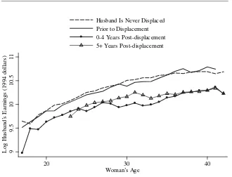
Age-husband’s Earnings Profile by Husbands’ Displacement Status
Notes: Data are from the 1968–1995 waves of the PSID, limited to ever married women. Averages cal-culated using less than 40 observations are not plotted. The profile for women 5Ⳮ years following a husband’s displacement begins later than the others because there are few women who are younger than 18 when their husband is first displaced.
profile for the control group. The solid line plots the profile for the displaced group but only uses person-years prior to a husband’s displacement—as such, it is the predisplacement profile of husbands’ earnings. These two profiles are nearly identical which suggests that, at any given age, the average predisplacement husbands’ earn-ings of the treated group are very close to the husbands’ earnearn-ings of the control group. The figure also shows profiles for women using person-years zero to four years following the shock and five or more years following the shock. Both of these profiles lie below the first two, demonstrating the loss in husbands’ earnings resulting from displacements. Further, the fact that the two post-displacement profiles are similar indicates the persistence of the shock.
con-0
.1
.2
.3
.4
P
roba
b
ilit
y
of H
av
ing
a C
h
il
d
20 30 40
Woman’s Age
Husband Is Never Displaced Prior to Displacement 0-4 Years Post-displacement 5+ Years Post-displacement
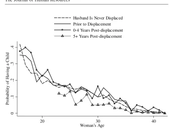
Figure 2
Age-probability of Conception Profile by Husbands’ Displacement Status Notes: Same as Figure 1.
trols while the profiles converge as women near the end of their childbearing years. This suggests that the impact of an income shock is largely about timing as the controls “catch up” in later years.
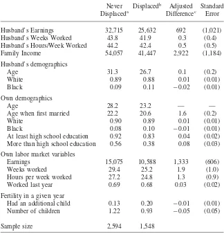
Table 1 presents sample means. For time-varying variables, the means are cal-culated using all person-year observations for the control group and person-years three or more years prior to the husband’s first displacement for the displaced group. This comparison is motivated by the idea that the predisplacement characteristics of women in the treatment group should be similar to the characteristics of women in the control group if husbands’ displacements are exogenous. However, because this sample selection artificially reduces the average age of the displaced group, the means are not informative for time-varying variables. To remedy this issue, the third column calculates the estimated difference, with controls for age and year fixed effects for time-varying variables.
The racial makeup of the women and their husbands is roughly the same across groups. Approximately 90 percent of the sample is white and 10 percent is black. The average age at the time of first marriage is 22.2 for the control group which is 1.6 years later than the average for the displaced group. Both groups of women are about three years younger than their first husband.
0
1
2
N
u
m
b
er
o
f C
h
il
d
ren
20 30 40
Woman’s Age
Husband Is Never Displaced Prior to Displacement 0-4 Years Post-displacement 5+ Years Post-displacement
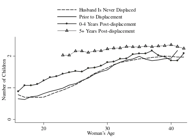
Figure 3
Age-children Profile by Husbands’ Displacement Status Notes: Same as Figure 1.
year. After making the appropriate adjustment, the differences in husbands’ earnings, weeks worked, and hours worked per week are not statistically significant. Further, the women in the two groups have similar numbers of children and probabilities of having additional children. At the same time, there is evidence that the controls are more educated than women in the displaced group—they are eight percentage points more likely to have more than a high school education after adjusting for their age and year. Given the educational disparity, it is not surprising that control women’s average adjusted earnings and family income are $1,333 and $2,929 greater than those in the displacement group, respectively. The differences in adjusted weeks worked per year, adjusted hours worked per week, and the adjusted probability of working are not statistically significant at the five percent level.
Table 1
Women’s Sample Means By Husbands’ Displacement Status
Never Displaceda
Displacedb Adjusted
Differencec
Standard Error
Husband’s Earnings 32,715 25,632 692 (1,021)
Husband’s Weeks Worked 43.8 41.9 0.3 (0.4)
Husband’s Hours/Week Worked 44.2 42.4 0.5 (0.5)
Family Income 54,057 41,447 2,922 (1,184)
Husband’s demographics
Age 31.3 26.7 0.1 (0.2)
White 0.89 0.88 0.01 (0.01)
Black 0.09 0.11 ⳮ0.02 (0.01)
Own demographics
Age 28.2 23.2 — —
Age when first married 22.2 20.6 1.6 (0.2)
White 0.90 0.89 0.01 (0.01)
Black 0.08 0.10 ⳮ0.01 (0.01)
At least high school education 0.92 0.83 0.04 (0.02)
More than high school education 0.56 0.38 0.08 (0.03)
Own labor market variables
Earnings 15,075 10,588 1,333 (606)
Weeks worked 29.4 25.2 1.9 (1.0)
Hours per week worked 27.2 24.8 1.3 (0.9)
Worked last year 0.69 0.68 0.03 (0.02)
Fertility in a given year
Had an additional child 0.13 0.20 ⳮ0.01 (0.01)
Number of children 1.22 0.93 ⳮ0.05 (0.05)
Sample size 2,594 1,548
Notes: Means and difference are weighted using the family weight in the last year with first husband. Money values are in 1994 dollars.
a. For time-varying variables, averages include all observations for women who never have a displaced spouse.
b. For time varying variables, averages use data for 3 or more years prior to displacement for women with a displaced spouse.
c. For time-varying variables, the difference is adjusted using age and year fixed effects. Standard errors are clustered on the individual.
B. Estimated Impact of Displacements on Husbands’ Earnings
women’s earnings if the change in women’s earnings is driven by changes in fertility. Further, theoretical models often predict that different sources of income will have different impacts on fertility. Again, the most important distinction tends to be be-tween women’s earnings and other sources of income and, for this reason, empirical studies often focus on male earnings as the measure of family income.
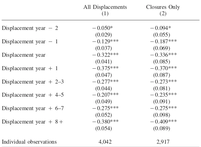
Column 1 of Table 2 presents regression estimates of the effect of a displacement on husbands’ log earnings.18 The estimates are based on a model with individual
fixed effects, year fixed effects, and a quadratic in the husband’s age in addition to the set of displacement indicators (Equation 1). Like previous studies, I find evidence that the immediate impact and the long-term impact are both large. The coefficient on the indicator for one year following the displacement suggests that earnings are reduced by 31.3 percent.19The estimated impacts over the subsequent years suggest
very little recovery. In fact, while not very precise, the estimated impact eight or more years following the displacement is as large as the estimated impact in the year following the displacement.20
Like other studies, I also find that men’s earnings begin to fall below their ex-pected levels shortly before the displacement occurs. My estimates imply a 12.1 percent reduction in the year prior to the displacement. Given that many displaced workers initial jobs are in distressed firms, this finding is not surprising. While the displacement literature provides little evidence of the mechanism driving this result, potential explanations include wage stagnation, reduced overtime, and temporary layoffs.
To some extent, the fact that earnings fall below their expected levels before the job loss occurs raises a question about whether displacements might be a function of an individual’s productivity. On the other hand, there is only weak evidence that they begin to fall below their expected levels two years prior to the job loss and, in results not shown, I have found no evidence that they begin to fall three years prior to the job loss. Further, the pattern is the same if I focus only on displacements that occur due to a plant or business closing, as in column 2. Specifically, women whose husbands’ displacements are due to being laid off or fired are not used in this analysis and the estimates still indicate that earnings drop below their expected levels in the year prior to the displacement.
Finally, the estimated impacts on husbands’ weeks worked, women’s earnings, and women’s weeks worked are displayed in Table A in the appendix. These esti-mates suggest that the long-term impact on husbands’ earnings is largely driven by reduced wages since the long-term impact on his weeks worked is small. Like Ste-phens (2002), I find that women work more following a husband’s displacement.
18. Note that, since the analysis is from the perspective of the woman, it does not track a husband’s earnings if they are in different households and does include a new husband’s earnings if the woman remarries.
19. The percentage effect on earnings is computed ase␦ⳮ1.
Table 2
Estimated Impact of Displacement on Husband’s Log Earnings
All Displacements (1)
Closures Only (2)
Displacement yearⳮ2 ⳮ0.050* ⳮ0.094*
(0.029) (0.055)
Displacement yearⳮ1 ⳮ0.129*** ⳮ0.187***
(0.037) (0.069)
Displacement year ⳮ0.322*** ⳮ0.336***
(0.041) (0.085)
Displacement yearⳭ1 ⳮ0.375*** ⳮ0.370***
(0.047) (0.087)
Displacement yearⳭ2–3 ⳮ0.277*** ⳮ0.273***
(0.044) (0.081)
Displacement yearⳭ4–5 ⳮ0.207*** ⳮ0.235***
(0.049) (0.091)
Displacement yearⳭ6–7 ⳮ0.275*** ⳮ0.275***
(0.052) (0.098)
Displacement yearⳭ8Ⳮ ⳮ0.380*** ⳮ0.409***
(0.054) (0.089)
Individual observations 4,042 2,917
Notes: All regressions include individual fixed effects, year fixed effects, and a quadratic in husband’s age. The omitted category is never having a displaced husband or three or more years prior to a husband’s displacement.
Standard error estimates, clustered on the individual, are displayed in parentheses. Regressions are weighted using the family weight from the last year women are observed with their first husband.
* significant at 10 percent; ** significant at 5 percent; *** significant at 1 percent
These results confirm that a husband’s job displacement has a large permanent impact on his earnings and suggest that the reduction is driven mostly by reduced wages rather than reduced work activity. Because the income shock has such im-portant impacts on a couple’s labor market outcomes, it would not be surprising to find impacts on fertility decisions. These impacts are explored in the next section.
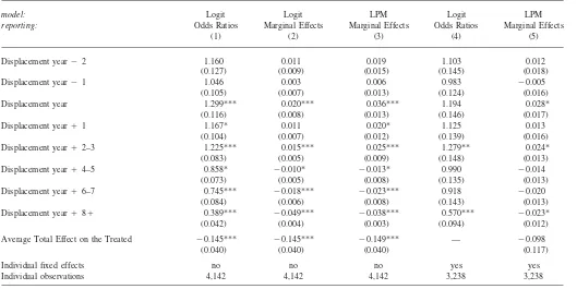
C. Estimated Impact of a Husband’s Displacement on Fertility
Lindo
317
model: Logit Logit LPM Logit LPM
reporting: Odds Ratios
(1)
Marginal Effects (2)
Marginal Effects (3)
Odds Ratios (4)
Marginal Effects (5)
Displacement yearⳮ2 1.160 0.011 0.019 1.103 0.012
(0.127) (0.009) (0.015) (0.145) (0.018)
Displacement yearⳮ1 1.046 0.003 0.006 0.983 ⳮ0.005
(0.105) (0.007) (0.013) (0.124) (0.016)
Displacement year 1.299*** 0.020*** 0.036*** 1.194 0.028*
(0.116) (0.008) (0.013) (0.146) (0.017)
Displacement yearⳭ1 1.167* 0.011 0.020* 1.125 0.013
(0.104) (0.007) (0.012) (0.139) (0.016)
Displacement yearⳭ2–3 1.225*** 0.015*** 0.025*** 1.279** 0.024*
(0.083) (0.005) (0.009) (0.148) (0.013)
Displacement yearⳭ4–5 0.858* ⳮ0.010* ⳮ0.013* 0.990 ⳮ0.014
(0.073) (0.005) (0.008) (0.135) (0.013)
Displacement yearⳭ6–7 0.745*** ⳮ0.018*** ⳮ0.023*** 0.918 ⳮ0.020
(0.084) (0.006) (0.008) (0.143) (0.013)
Displacement yearⳭ8Ⳮ 0.389*** ⳮ0.049*** ⳮ0.038*** 0.570*** ⳮ0.023*
(0.042) (0.004) (0.003) (0.094) (0.012)
Average Total Effect on the Treated ⳮ0.145*** ⳮ0.145*** ⳮ0.149*** — ⳮ0.098
(0.040) (0.040) (0.040) (0.117)
Individual fixed effects no no no yes yes
Individual observations 4,142 4,142 4,142 3,238 3,238
Notes: The dependent variable is an indicator for having a child in a given year. All columns include age fixed effects and a quadratic in the year. The omitted category is never having a displaced husband or three or more years prior to a husband’s displacement. Standard error estimates, clustered on the individual, are displayed in parentheses. Regressions are weighted using the family weight from the last year women are observed with their first husband. The estimation of the average total effect is described in Section V.C. The odds ratios in columns 1 and 4 are e—an odds ratio of one indicates no effect, greater than one indicates increased odds, and less than
one indicates reduced odds.
same controls. Each set of estimates implies that the odds of having a child are significantly higher in the first four years following the job loss before the effect reverses and the odds are significantly reduced. That is, the negative shock to a husband’s earnings accelerates the timing of children.
A possible concern with these estimates is that the estimated impact might arise as a result of unobservable characteristics that are related to both fertility and the probability of having a displaced husband. If such unobservable characteristics exist, then models that include individual fixed effects will provide unbiased estimates if they are fixed over time. Column 4 presents odds ratios based on an individual fixed effects logit model (Equation 3) while Column 5 presents coefficient estimates based on a linear probability model with individual fixed effects (in addition to the controls used in Columns 1–3). Like the estimates based on the models without individual fixed effects, these estimates suggest an increase in the odds of having children in the years immediately following the displacement and a subsequent reduction in the odds many years following the event. The magnitudes are slightly smaller and, not surprisingly, the standard error estimates are larger in these models due to both the individual fixed effects and the fact that individuals without variation in the depen-dent variable cannot be used in a fixed effects logit model.21Nevertheless, the
in-creased odds soon after the event and the reduced odds eight or more years following the event are statistically significant.
While the estimated dynamic fertility response does not itself tell us whether the net impact on fertility will be positive or negative, the estimated model can be used to estimate the net fertility impact with the approach described in Section VC. For a woman who has a husband displaced at some time, her predicted total (post-displacement) fertility can be obtained by adding up her predicted probabilities of having a child in each year following the displacement. Similarly, a counterfactual can be estimated by the same method after turning the displacement indicators off. The average difference between these estimates provides an estimate of the average impact on the total fertility of the treated.
These estimates, based on each of the models discussed above, are displayed in Table 4 beneath the estimates of the dynamic response. All of the estimates suggest that a husband’s job loss has a net negative impact on fertility. The estimated effects based on the models without individual fixed effects are statistically significant, indicating a 0.14 reduction in the total number of children. While predicted proba-bilities cannot be obtained from the fixed effects logit model, the linear probability model with individual fixed effects indicates that a husband’s displacement reduces total fertility by 0.10 children. However, the individual fixed effects greatly reduce the precision of the estimate and it is not statistically significant.
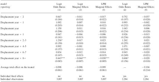
Table 4 presents estimates that focus on the effects of a husband’s displacement resulting from a plant or business closure. While omitting women whose husbands lost their jobs due to being laid off or fired substantially reduces the sample of women experiencing a husband’s displacement (from 1,548 to 413), the advantage of this approach is that job losses resulting from plant or business closures are more
Lindo
319
model: Logit Logit LPM Logit LPM
reporting: Odds Ratios
(1)
Marginal Effects (2)
Marginal Effects (3)
Odds Ratios (4)
Marginal Effects (5)
Displacement yearⳮ2 0.847 ⳮ0.011 ⳮ0.017 0.752 ⳮ0.037
(0.184) (0.014) (0.022) (0.197) (0.028)
Displacement yearⳮ1 1.092 0.007 0.010 0.993 ⳮ0.002
(0.203) (0.014) (0.022) (0.232) (0.028)
Displacement year 1.150 0.011 0.016 1.043 0.006
(0.206) (0.015) (0.022) (0.234) (0.028)
Displacement yearⳭ1 0.947 ⳮ0.004 ⳮ0.006 0.926 ⳮ0.013
(0.181) (0.013) (0.020) (0.236) (0.028)
Displacement yearⳭ2–3 1.236* 0.017 0.023 1.262 0.021
(0.150) (0.010) (0.014) (0.255) (0.022)
Displacement yearⳭ4–5 0.992 ⳮ0.001 0.000 1.071 ⳮ0.007
(0.157) (0.011) (0.015) (0.239) (0.021)
Displacement yearⳭ6–7 0.834 ⳮ0.012 ⳮ0.014 0.943 ⳮ0.020
(0.167) (0.013) (0.015) (0.249) (0.021)
Displacement yearⳭ8Ⳮ 0.443*** ⳮ0.044*** ⳮ0.030*** 0.606* ⳮ0.020
(0.083) (0.007) (0.005) (0.156) (0.018)
Average total effect on the treated ⳮ0.098 ⳮ0.098 ⳮ0.099 — ⳮ0.104
(0.061) (0.061) (0.061) (0.214)
Individual fixed effects no no no yes yes
Individual observations 3,007 3,007 3,007 2,284 2,284
Notes: Same as Table 3.
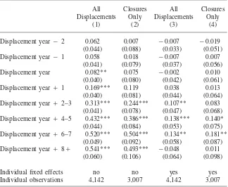
plausibly exogenous than those resulting from being laid off or fired. These estimates provide less evidence of an increase in the odds of having a child in the year the job loss occurs but continue to indicate increased odds of having children 2–3 years following the event and reduced odds of having children six or more years after the event. Further, the estimates indicate that a husband’s displacement reduces total fertility by approximately 0.10 children. While the estimates based on this sample are rarely statistically significant as a result of the small sample size, they lend confidence to the results based on the full sample which are similar but more precise. To further explore the net effect of a job displacement on fertility, Table 5 uses the cumulative number of children born as of each given year as the dependent variable instead of an indicator for having a child in a given year. Here, the coef-ficients on the displacement indicators can be thought of as measuring the cumulative impact on the “stock” of children whereas the estimates presented in Table 4 mea-sured the impact on the “flow.” As with the prior estimates, age fixed effects and a quadratic in year are included in the models. Although the estimates that do not control for individual fixed effects (Columns 1 and 2) suggest that displacements lead to a long-term increase in the number of children, estimates controlling for individual fixed effects (Columns 3 and 4) are similar to the prior estimates.22The
positive coefficients on indicators for 2–3, 4–5, and 6–7 years following the dis-placement imply that the disdis-placement causes an increase in the number of children soon after the event while the coefficient on the indicator for eight or more years following the event implies that the increase is only temporary.
It should be noted that the estimated coefficient on the indicator for eight or more years after a husband’s job loss suggests that the long-term impact on fertility is smaller than the prior estimates (and positive when only closures are considered). However, this is due to the fact that this coefficient combines the cumulative impact as of 8–9 years after the event with the cumulative impact at later years. If the vector of displacement indicators instead includes indicators for 8–9 years following the event and 10 or more years following the event, the coefficient on 10 or more years following the event is negative for both samples.23
VII. Discussion
These results suggest that negative income shocks have substantive impacts on the timing of fertility. The overall pattern, with increases in fertility in the years immediately following a husband’s job loss and reductions many years later, is robust—the pattern is seen in both logit models and linear probability models and using both a broad definition of displacement and a definition that only includes plant or business closings.
This pattern of estimates is consistent with dynamic models of fertility. In these models, credit-constrained households have an incentive to delay childbearing until
22. As one would expect, the estimates that do not control for individual fixed effects mirror the graphical analysis of means in Figure 3.
Table 5
Estimated Impact of a Husband’s Displacement on the Cumulative Number of Children
All Displacements
Closures Only
All Displacements
Closures Only
(1) (2) (3) (4)
Displacement yearⳮ2 0.062 0.007 ⳮ0.007 ⳮ0.019
(0.044) (0.088) (0.033) (0.051)
Displacement yearⳮ1 0.058 0.018 ⳮ0.007 0.007
(0.041) (0.079) (0.037) (0.056)
Displacement year 0.082** 0.075 ⳮ0.002 0.010
(0.040) (0.080) (0.042) (0.061)
Displacement yearⳭ1 0.169*** 0.119 0.038 0.013
(0.040) (0.081) (0.044) (0.064)
Displacement yearⳭ2–3 0.313*** 0.244*** 0.107** 0.083
(0.041) (0.078) (0.047) (0.068)
Displacement yearⳭ4–5 0.432*** 0.386*** 0.138*** 0.140*
(0.044) (0.084) (0.053) (0.075)
Displacement yearⳭ6–7 0.520*** 0.504*** 0.134** 0.181**
(0.049) (0.092) (0.058) (0.087)
Displacement yearⳭ8Ⳮ 0.541*** 0.493*** ⳮ0.048 0.011
(0.060) (0.106) (0.064) (0.098)
Individual fixed effects no no yes yes
Individual observations 4,142 3,007 4,142 3,007
Notes: The dependent variable is the cumulative number of children the woman has had to date in a given year. All columns include age fixed effects and a quadratic in the year. The omitted category is never having a displaced husband or three or more years prior to a husband’s displacement. Standard error estimates, clustered on the individual, are displayed in parentheses. Regressions are weighted using the family weight from the last year women are observed with their first husband.
* significant at 10 percent; ** significant at 5 percent; *** significant at 1 percent
the husband’s earnings are higher. Because job displacements reduce a husband’s earnings growth, it then reduces the incentive to delay children. It is important to note that this theoretical prediction involves the slope of a husband’s earnings tra-jectory rather than the absolute level of his earnings. A different type of shock that affected a husband’s earnings in a different manner might have different effects.24
Another possible explanation for the observed pattern involves the effect of dis-placements on husbands’ time. While the reduction in work activity immediately following a job loss is not especially large, it might make for a relatively convenient
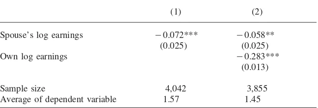
Table 6
Estimated Cross-sectional Relationship Between Spouse’s Earnings and the Number of Children
(1) (2)
Spouse’s log earnings ⳮ0.072*** ⳮ0.058**
(0.025) (0.025)
Own log earnings ⳮ0.283***
(0.013)
Sample size 4,042 3,855
Average of dependent variable 1.57 1.45
Notes: Regressions include age and year fixed effects. Standard error estimates, clustered on the individual, are displayed in parentheses. Regressions are weighted using the family weight from the last year women are observed with their first husband.
* significant at 10 percent; ** significant at 5 percent; *** significant at 1 percent
time for a woman to have a child. It is unfortunate that this hypothesis cannot be ruled out because, if true, the implications for economic theory are rather serious— as Hotz, Klerman, and Willis (1997) explain in an in-depth review of the literature, with all of the various features that have been integrated into lifecycle models of household fertility, none consider the time allocation decisions of fathers.
My estimated impact on total fertility is very similar to that of Heckman and Walker (1990), although it is not statistically significant when individual fixed effects are included. Heckman and Walker estimate that a 12 percent increase in male wages increases total fertility by 0.05 children and I find that a long-term 32 percent re-duction in husbands’ earnings is accompanied by a 0.10 rere-duction in total fertility. My estimates provide an opportunity to assess of the degree to which the cross-sectional relationship between income and fertility mischaracterizes the causal re-lationship. Table 6 presents estimates of the cross-sectional rere-lationship. Column 1 shows the coefficient from a regression of the current number of children on hus-bands’ log earnings. Both age and year fixed effects are included in the model to isolate the cross-sectional variation in the longitudinal data. As is commonly seen in cross-sectional data, the relationship is negative. Column 2, which controls for women’s log earnings, continues to indicate a negative relationship. Taking the stan-dard approach of using husbands’ earnings as the income measure, these estimates suggest that the income elasticity is betweenⳮ0.04 andⳮ0.05.25,26
In contrast, using the estimated long-term impact on husbands’ earnings (ⳮ31.6 percent), the average total impact on the fertility of the treated (ⳮ0.10), and the average total observed fertility for the treated (2.06), I obtain an estimated income
25. Analysis focusing solely on women who have a displaced husband yields similar results.
elasticity of 0.15. This estimate likely understates the true elasticity since the long-term impact on family income will be less than the impact on husbands’ earnings (which are only a share of income).
This finding raises the question: if the causal relationship between husband’s earn-ings and fertility is truly positive, why is the correlation negative? More specifically, what type of model is consistent with such phenomena? Extending the basic model to consider child quality is not sufficient since the causal relationship and the cor-relation are the same in such a model. A model that incorporates the time cost of children and assortative matching of husbands and wives, however, can solve the puzzle. In such a model, a high wage couple could have a high income but not have many children because of the high value of the wife’s time. This would produce a negative correlation between husband’s earnings and fertility in the cross-section but would not preclude a couple from having fewer (more) children in response to a reduction (increase) in income.27
VIII. Conclusion
In this paper, I have examined the impact on fertility of a large negative shock to a husband’s earnings. Consistent with dynamic models in which children produce a flow of benefits and credit markets are incomplete, I find that a reduction in a husband’s earnings growth accelerates fertility. I also find evidence that a large negative income shock reduces completed fertility, although it is not statistically significant when individual fixed effects are included in the model. This estimate implies an income elasticity of 0.15 which stands in stark contrast to the negative correlation between fertility and husbands’ earnings observed in cross-sec-tional data. While the quantity-quality model cannot itself explain these seemingly opposed relationships, a model with assortative matching of spouses that incorpo-rates the time cost of children can.
Policy implications should depend on several factors. Clearly, whether or not it is desirable for job losses to reduce fertility depends on a given society’s current and targeted fertility rates. Any policy designed to affect the link between fertility and displacement should also take into account the outcomes of the children born following a father’s job loss. While the literature shows that children suffer long-term consequences of parental displacements, little is known about the effects on children who are born after a parent’s job loss.28More research along these lines is
needed.
More broadly, understanding the causal effect of income on fertility is important for any policy prescription that involves income shocks. The positive relationship implied by my estimates suggests that poverty relief programs could unintentionally promote fertility. Policy projections that ignore this fertility response will overstate the expected impact of financial assistance on living standards.
The
Journal
of
Human
Resources
Appendix Table 1
Estimated Impact of a Husband’s Displacement on Additional Labor Market Outcomes
Husband’s Weeks/Year Worked Women’s Log Earnings Women’s Weeks/Year Worked
All Displacements
Closures Only
All Displacements
Closures Only
All Displacements
Closures Only
(1) (2) (3) (4) (5) (6)
Displacement yearⳮ2 ⳮ0.974* ⳮ1.327 ⳮ0.022 ⳮ0.086 0.220 0.468
(0.550) (0.857) (0.057) (0.097) (0.931) (1.705)
Displacement yearⳮ1 ⳮ1.495** ⳮ0.502 0.026 ⳮ0.142 1.776* 1.005
(0.587) (0.964) (0.065) (0.116) (0.954) (1.642)
Displacement year ⳮ5.749*** ⳮ5.005*** 0.035 ⳮ0.049 1.166 ⳮ1.268
(0.617) (1.091) (0.061) (0.109) (0.943) (1.687)
Displacement yearⳭ1 ⳮ5.367*** ⳮ4.948*** 0.026 ⳮ0.139 1.763* 0.683
(0.682) (1.013) (0.064) (0.117) (1.003) (1.719)
Displacement yearⳭ2–3 ⳮ2.994*** ⳮ3.532*** 0.050 ⳮ0.117 2.516** 0.446
(0.645) (1.055) (0.064) (0.114) (1.017) (1.705)
Displacement yearⳭ4–5 ⳮ1.339** ⳮ1.873 0.045 ⳮ0.025 2.895** 1.449
(0.665) (1.165) (0.072) (0.124) (1.143) (1.941)
Displacement yearⳭ6–7 ⳮ1.809*** ⳮ1.642 0.086 ⳮ0.049 3.186** 0.891
(0.702) (1.156) (0.081) (0.135) (1.238) (2.138)
Displacement yearⳭ8Ⳮ ⳮ2.096*** ⳮ3.172*** 0.204** 0.039 7.288*** 4.139**
(0.761) (1.149) (0.085) (0.136) (1.307) (2.054)
Individual Observations 4,141 3,006 3,980 2,870 4,141 3,006
Notes: All regressions include individual fixed effects, year fixed effects, and a quadratic in husband’s age. The omitted category is never having a displaced husband or three or more years prior to a husband’s displacement. Standard error estimates, clustered on the individual, are displayed in parentheses. Regressions are weighted using the family weight from the last year women are observed with their first husband.
References
Amialchuk, Aliaksandr. 2006. “Timing of the Response of Household Fertility Decisions to
Husband’s Earnings Shocks on the Timing of Fertility.” University of Toledo. Unpublished.
Angrist, Joshua D., and William N. Evans. 1998. “Children and Their Parents’ Labor
Supply: Evidence from Exogenous Variation in Family Size.”American Economic
Review88(3):450–77.
Becker, Gary S. 1960. “An Economic Analysis of Fertility.” In Demographic and Economic Change in Developed Countries, a conference of the Universities-National Bureau Committee for Economic Research, 209–31. Princeton: Princeton University Press.
———. 1965. “A Theory of the Allocation of Time.”The Economic Journal75(299):493–
517.
———. 1991.A Treatise on the Family. Cambridge: Harvard University Press.
Becker, Gary S., and H. Gregg Lewis. 1973. “On the Interaction between the Quantity and
Quality of Children.”Journal of Political Economy81(2): S279–S288.
Bjo¨rklund, Anders. 1985. “Unemployment and Mental Health: Some Evidence from Panel
Data.”Journal of Human Resources20(4):469–83.
Black, Sandra E., Paul J. Devereux, and Kjell G. Salvanes. 2008. “Staying In the Classroom and Out of the Maternity Ward? The Effects of Compulsory Schooling Laws on Teenage
Births.”Economic Journal118:1025–54.
Browning, Martin, Ann Moller Dano, and Eskil Heinesen. 2006. “Job Displacement and
Stress-Related Health Outcomes.”Health Economics15(10):1061–75.
Chan, Sewin, and Ann Huff Stevens. 1999. “Employment and Retirement Following a
Late-Career Job Loss.”American Economic Review, Papers and Proceedings89(2):211–16.
Charles, Kerwin Kofi, and Melvin Stephens, Jr. 2004. “Job Displacement, Disability, and
Divorce.”Journal of Labor Economics20(3):489–522.
de la Rica, Sara. 1995. “Evidence of Pre-Separation Earnings Losses in the Displaced
Worker Survey.”Journal of Human Resources30(3):610–21.
Dehejia, Rajeev, and Adriana Lleras-Muney. 2004. “Booms, Busts, and Babies’ Health.”
Quarterly Journal of Economics119(3):1091–1130.
Dickert-Conlin, Stacy, and Amitabh Chandra. 1999. “Taxes and the Timing of Births.”
Journal of Political Economy107(1): 161–177.
Duclos, Edith, Pierre Lefebvre, and Phillip Merrigan. 2001. “A Natural Experiment on the Economics of Storks: Evidence on the Impact of Differential Family Policy on Fertility Rates in Canada.” CREFE Working Paper 136, Universite´ du Que´bec a` Montre´al. Gans, Joshua S., and Andrew Leigh. 2007. “Born on the First of July: An (Un)natural
Experiment in Birth Timing.”Journal of Public Economics. Forthcoming.
Eliason, Marcus, and Donald Storrie. 2006. “Lasting or Latent Scars? Swedish Evidence on
the Long-Term Effects of Job Displacement.”Journal of Labor Economics24(4): 831–
856.
Heckman, James J., and Robert J. Willis. 1975. “Estimation of a Stochastic Model of
Reproduction: An Econometric Approach.” InHousehold Production and Consumption,
ed. Nestor E. Terleckyj, 99–146. New York: Columbia University Press.
Heckman, James J., and James R. Walker. 1990. “The Relationship Between Wages and Income and the Timing and Spacing of Births: Evidence from Swedish Longitudinal
Data.”Econometrica58(6): 1411–441.
Hotz, Joseph V., Jacob A. Klerman, and Robert J. Willis. 1997. “The Economics of Fertility
in Developed Countries.” InHandbook of Population and Family Economics, ed. Mark
Hoynes, Hilary W. 1997. “Work, Welfare, and Family Structure: What Have We Learned?” InFiscal Policy: Lessons from Economic Research, ed. Alan J. Auerbach, 101–46. Cambridge: MIT Press.
Jacobson, Louis S., Robert J. LaLonde, and Daniel G. Sullivan. 1993. “Earnings Losses of
Displaced Workers.”American Economic Review83(4):685–709.
Jones, Larry E., Alice Schoonbroodt, and Miche`le Tertilt. 2008. “Fertility Theories: Can They Explain the Negative Fertility-Income Relationship?” NBER Working Paper 14266. Cambridge: National Bureau of Economic Research.
Jones, Larry E., and Miche`le Tertilt. 2007. “An Economic History of Fertility in the U.S.:
1826–1960.” InThe Handbook of Family Economics, ed. Peter Rupert. Forthcoming.
Kletzer, Lori G., and Robert W. Fairlie. 2003. “The Long-Term Costs of Job Displacement
for Young Adult Workers.”Industrial and Labor Relations Review56(4):682–98.
Manski, Charles F., and John D. Straub. 2000. “Worker Perceptions of Job Insecurity in the
Mid-1990s: Evidence from the Survey of Economic Expectations.”Journal of Human
Resources35(3):447–79.
McCrary, Justin, and Heather Royer. 2006. “The Effect of Maternal Education on Fertility and Infant Health: Evidence from School Entry Policies Using Exact Date of Birth.” NBER Working Paper 12329. Cambridge: National Bureau of Economic Research. Merrigan, Phillip, and Yvan St-Pierre. 1998. “An Econometric and Neoclassical Analysis of
the Timing and Spacing of Births in Canada from 1950–1990.”Journal of Population
Economics11(1):29–51.
Milligan, Kevin. 2005 “Subsidizing the Stork: New Evidence on Tax Incentives and
Fertility.”Review of Economics and Statistics87(3):539–55.
Mincer, Jacob. 1963. “Market Prices, Opportunity Costs, and Income Effects.” In
Measurement in Economics: Studies in Mathematical Economics in Honor of Yehuda Grunfeld, ed. Carl F. Christ et al., 67–82. Stanford: Stanford University Press.
Moffitt, Robert A. 1998. “The Effect of Welfare on Marriage and Fertility.” InWelfare, the
Family, and Reproductive Behavior, ed. Robert A. Moffitt, 50–97. Washington, D.C.: National Research Council.
Newman, John L. 1988. “A Stochastic Dynamic Model of Fertility.” InResearch in
Population Economics6, ed. T. Paul Schultz, 48–61. Greenwich: JAI Press.
Oreopoulos, Philip, Marianne E. Page, and Ann Huff Stevens. 2008. “The Intergenerational
Effects of Worker Displacement.”Journal of Labor Economics26(3):455–83.
Page, Marianne E., Ann Huff Stevens, and Jason M. Lindo. 2009. “Parental Income Shocks
and Outcomes of Disadvantaged Youth in the United States.” InAn Economic
Perspective on the Problems of Disadvantaged Youth, ed. Jonathan Gruber, 213–35. Chicago: University of Chicago Press.
Rhum, Christopher J. 1991. “Are Workers Permanently Scarred by Job Displacements?”
American Economic Review81(1):165–88.
Schultz, T. Paul. 1985. “Changing World Prices, Women’s Wages and the Fertility
Transition: Sweden, 1860–1910.”Journal of Political Economy93(6):1126–54.
Stephens, Jr., Melvin 2001. “The Long-run Consumption Effects of Earnings Shocks.”
Review of Economics and Statistics83(1):28-–36.
———. 2002. “Worker Displacement and the Added Worker Effect.”Review of Economics
and Statistics20(2):504–36.
———. 2004. “Job Loss Expectations, Realizations, and Household Consumption
Behavior.”Review of Economics and Statistics86(1):253–69.
Stevens, Ann Huff. 1997. “Persistent Effects of Job Displacement: The Importance of
Multiple Job Losses.”Journal of Labor Economics15(1):165–88.
Stromova, Masha. 2007. “Russian Region to Host Day of Conception.”Washington Post
Topel, Robert. 1990. “Specific Capital and Unemployment: Measuring the Costs and
Consequences of Job Loss.”Carnegie-Rochester Conference Series on Public Policy
33(1):181–214.
Whittington, Leslie A., James Alm, and H. Elizabeth Peters. 1990. “Fertility and the
Personal Exemption: Implicit Pronatalist Policy in the United States.”American
Economic Review80(3):545–56.
Willis, Robert J. 1973. “A New Approach to the Economic Theory of Fertility Behavior.”
Journal of Political Economy81(2): S14–S64.
Wolpin, Kenneth I. 1984. “An Estimable Dynamic Stochastic Model of Fertility and Child
Mortality.”Journal of Political Economy92(5):852–74.
Zhang, Junsen, Jason Quan, and Peter Van Meerbergen. 1994. “The Effect of Tax-Transfer
Policies on Fertility in Canada, 1921–1988.”Journal of Human Resources29(1):181–