Impact of Financial Development on Income Inequality and Poverty in
ASEAN
Ridwan Nurazia, Berto Usmanb
Abstract: This study investigates the effect of financial development on income inequality and poverty in the context of the ASEAN (Association of Southeast Asian Nations) economy. Investigating the relationship of financial development to economic variables has attracted much attention among researchers and practitioners. Nonetheless, prior studies have resulted in conflicted and inconclusive output concerning the a priori effect of finance on the general economic progress. Therefore, by employing the longitudinal panel data analysis, we provide empirical evidence with more specific cases on the link between the finance-inequality and finance-poverty nexus. Utilising panel data analysis for a sample of five ASEAN countries (Indonesia, Malaysia, Philippines, Thailand, and Vietnam from 2007 to 2015), we investigate our proposed empirical model.
Hereby, we use four financial dimensions as the proxy for financial development (financial access, financial deepening, financial efficiency, and financial stability). The Gini index and poverty gap are considered proxies of income inequality and poverty. Our results report that financial development by employing four financial dimensions contribute more to the variability of the poverty gap rather than the Gini index ratio.
Also, we document that the surrogate indicators of financial access, financial deepening, financial efficiency are statistically associated with the poverty gap. On the other hand, no association is found between the proxy of financial development and income inequality.
Keywords: Financial development; income inequality; poverty JEL Classification: G1; G2; H50
Article Received: 8 March 2018; Article Accepted: 19 December 2018
1. Introduction
Inspired by studies on inequality and poverty, this study identifies the contribution of financial development on the income inequality and poverty in ASEAN (Association of South-East Asian Nations) economies. The paper focuses on investigating whether several channels of financial development act positively or negatively to the variance of income inequality and poverty.
a Department of Management, Faculty of Economics and Business, University of Bengkulu, Indonesia. Email: [email protected]
b Corresponding author. Department of Management, Faculty of Economics and Business, University of Bengkulu, Indonesia. Email: [email protected]
As documented by Naceur and Zhang (2016), prior theories on the effect of financial development on income inequality and poverty offer a conflicting prediction. In this regard, several researchers (Agnello, Mallick, & Sousa, 2012; Greenwood & Jovanovic, 1990; Nikoloski, 2013) noted that in one strand of literature, the effect of financial development on income distribution proposes an inverted U-shaped relationship. On the other hand, researchers (Galor & Moav, 2004; Galor & Zeira, 1993) posit a linear relationship between financial development on income distribution and poverty.
More precisely, empirical studies draw on numerous results on the study of income distribution and poverty, but the attempt to link this concept with finance is still scant. Among them, Bittencourt (2010) tests the causal-effect relationship between financial development and inequality. He reports that a deeper and more active financial sector alleviates the high inequality in the Brazilian economy. By employing specific time-series analysis from the 1980s to 1990s, he notes that the alleviation of the financial sector on the inequality emerges without a particular need for distortionary taxation.
Moreover, Jeanneney and Kpodar (2011) investigate the ability of financial development in reducing poverty. Their findings reveal that financial development helps to reduce the rate of poverty directly through the distribution effect. By focusing on developing countries, they confirm that the poor benefited from accessibility to the banking system.
Our study also focuses on highlighting and providing empirical evidence, in which the levels of inequality and poverty in Southeast Asian countries are significant across country and regions. As reported by Johansson and Wang (2014), the distribution of income varies significantly over time. This is also previously highlighted by Beck, Demirgüç-Kunt, and Levine (2007) who point out the presence of declining trend of inequality in some countries, but others at the same time also experience an increasing inequality. The conflicting patterns commonly showed by the different characteristics across country and time-variant factors. While the link between finance to income inequality and poverty is currently acknowledged, limited research has sought to comprehensively identify the potential relationship between the links of finance-inequality-poverty nexus.
This paper responds to calls to study finance-inequality and finance- poverty links. Also, it helps to distinguish between the conflicting view among the previous studies which documented inconclusive output between the relationship of finance-inequality and finance-poverty. By employing cross-country analysis in the ASEAN economy setting, financial development is considered to perform essential roles in the economic environment. Due to its importance, the contribution of financial development on income inequality and poverty is threefold. First, financial access as provided by the financial institution in terms of access to credit
creates more opportunity to enlarge benefits for the poor and the middle class, particularly through the investment channel in various productive activities. Second, regarding the presence of inflation and the probability of the ongoing possibility of hyperinflation happening, it can help governments better maintain the level of inflation. In this respect, the government can generate a substitution regarding the higher requirement of cash-in-advance constraints to the other instrument of credit (e.g., overdrafts, post-dated cheques, and credit cards). Third, when the government experiences high unemployment, particularly due to unpredictable macroeconomic instability, they can overcome this issue by improving access to credit and financial instruments that can smooth consumption during the short-time unemployment period.
Considering the specific issue of financial development and its association with income inequality and poverty, we focus more on investigating the association and contribution of the relationship among financial-inequality-poverty nexus in the ASEAN economy. We conjecture there might be a significant difference in the practices and phenomenon of financial development in the economy of developed and emerging countries.
In this respect, ASEAN members have shown similar characteristics that include the transition of its economy, persistent economic growth, and unneglected roles in the variability of the world economy as emerging markets. Due to this motive, we expect that the investigation in the context of emerging countries (i.e., Indonesia, Malaysia, Thailand, Philippine, and Vietnam) might behave differently due to varying economic circumstances and institutional conditions.
The remainder of our paper is organised as follows. The literature review and hypothesis development discuss the relevant literature and the procedure of hypothesis development concerning the main leading theories and prior studies. Research method provides the procedure and description of sample selection, data, and model specification. Results and discussion analyse the descriptive statistics and the empirical results derived from panel data analysis. Additional analysis is provided through the robustness test. The last section presents the discussion and overall result, which is inferred in the concluding remarks.
2. Literature Review and Hypothesis Development
2.1 The Association of Financial Development with Income Inequality In this section, we focus on investigating the association between financial development and income inequality. Due to the specific effect, which will be the primary predictor in this study, we also attempt to specify the link between financial development and income inequality through various
macroeconomic channels. The utilisation of macroeconomic variables has been identified by prior theoretical and empirical studies (Beck, Demirgüç- Kunt, & Levine, 2007; Claessens & Perotti, 2007; de Haan & Sturm, 2017;
Demirgüç-Kunt & Levine, 2009). Therefore, we employ the conceptual framework developed by Naceur and Zhang (2016) in which they applied macroeconomic variables to explain the variation of income inequality that is caused by the variability of financial development.
More precisely, we adopt critical mass theory (Schelling, 1971a, 1971b, 1978), which is commonly adopted for mapping social dynamics. Hereby, the underpinning idea of critical mass theory from the economic point of view relates to the sufficient number of adopters of innovation in a social system. In this respect, adopting financial innovation will achieve a specific rate within the social group. Therefore, the rate of self-adoption will be self- sustaining and is expected to generate a higher rate of the adopted innovation.
Given the nature of critical mass theory, it is highly considered that the idea of critical mass might be connected to the majority consensus in politics and economics. Small changes in the public consensus may lead to a change occurs in the political consensus. This change is mainly triggered by the majority-dependent of certain concept and idea coming from the public consensus, and be used as the media and tool in the political debates.
Notwithstanding the role of critical mass theory with our proposed idea, we argue that this theory could have been useful in explaining social dynamics and phenomenon, where the government as the standard setter creates policies which are mainly devoted to public interests. The logic is that the government decision to adopt higher financial development in fostering the economic growth and reducing inequality is considered collective action. Every part related to the government policies (stakeholders) should be aligned with a government objective. Therefore, prior study also employs the critical mass theory to describe the association between financial development and income inequality (Batuo, Guidi, &
Mlambo, 2007).
In this case, financial development is proxied by four specific financial dimensions, namely financial access, financial deepening, financial efficiency, and financial stability. These four dimensions expectedly show an association between finance and inequality links. For instance, Jauch and Watzka (2016) analyse the link between financial development and income inequality with an unbalanced dataset from the years 1960 to 2008. They find that of the 138 developed and developing countries, the utilisation of private credit as the proxy of financial development contradicts the a priori theory.
The findings report that financial development increases income inequality.
Otherwise, Hermes (2014) shows that there are relatively small negative effects of microfinance on the reduction of income inequality. Meaning that although the access to microfinance seemingly improves the relative income
position of the low-income people (poor), this improvement is deemed modest due to the relative utilisation of microfinance compare with the economy size of the countries. Law, Tan, and Azman-Saini (2014) further test the association between financial development and income inequality.
They reveal that financial development tends to reduce the level of income inequality if and only if the circumstance of a certain threshold level of institutional quality has been achieved already. This denotes that institutional quality plays a role in the nexus between the relationship of financial development and income inequality, in which better quality of finance triggers equal income distribution. Nonetheless, referring to the study of Demirgüç-Kunt and Levine (2009), they note that among many empirical studies, ambiguous predictions emerge since the inconclusive findings are still offering the mixed report about the impact of financial development on inequality (income distribution). This shows that the link between empirical research and theory in this line of research is still relatively weak (de Haan
& Sturm, 2017). Thus, according to the underlying theory and current literature, we formulate our hypothesis one as follows.
Hypothesis 1: Ceteris paribus, financial development is associated with income inequality
2.2 The Association of Financial Development with Poverty
Most of the literature highlights the relationship between finance and inequality, while the empirical investigation on the relationship between financial development and poverty is still scarce. Some studies suggest that financial instability worsen the circumstance of poverty (Jeanneney &
Kpodar, 2011). Jeanneney and Kpodar argue that the poor are more likely to be more vulnerable to banking crises than those who have a huge amount of capital. In this case, an indirect effect may appear due to the instability of economic growth and the rate of inflation induced by an unstable financial system. Moreover, Chakravarty and Pal (2013) specifically analyse the geographic penetration of banks and credit availability to boost the financial inclusion in India. They find that the social-banking policy has taken a big role in fostering the financial inclusion across the state in India during 1977- 1990. Given that, the axiomatic measures of financial inclusion, they utilised provide evidence of reducing inequality and poverty.
Another justification of the linear relationship between financial development and poverty is also previously highlighted by McKinnon (1974). The “conduit effect”1 might play a specific role in explaining the main function of money and capital. These two major factors (money and capital) are complementary when the real return on holding money increases (i.e., there is no useful distinction between the investors (firms) and the
savers (households) since they are deemed as an economic unit which confined to a self-financed). Thereby McKinnon (1974) argues that the desirability of holding cash balances from the perspective of the poor reduces the opportunity cost of saving internally. This condition is confirmed by the study of de Haan and Sturm (2017). Their study suggests that financial imperfections such as the transaction cost and the information could have bound the poor, which in this case is the lack of collateral and credit histories.
Given this circumstance, the credit constraint may benefit the poor.
Moreover, the recent study of Nkwoma, Jin, and Valenzuele (2018) points out that financial integration is beneficial in reducing market income inequality, but worsen net income inequality. This suggests that financial intermediation is found to be detrimental to net income inequality. They also document that independent access to finance has shown no relationship with income inequality.
The theoretical and empirical evidence so far suggests that the financial system provides unequal access to households and companies (Claessens &
Perotti, 2007). Natural economic reasons can be the triggering factors which initiate the un-optimum role of the financial system for all the stakeholders.
For instance, the high fixed cost in the process of offering the products of financial services may affect poverty negatively. Claessens and Perotti (2007), Johnson and Mitton (2003), Leuz and Oberholzer-Gee (2006) and Kamaludin and Usman (2018) further note that in a country with poor political constitution, the issue of unequal access is also caused by political influence. Hereby, the access to finance can only be experienced by certain groups. Due to the impact of the un-optimum role of financial development and the model of financial policies, the level of poverty cannot be reduced properly (Jeanneney & Kpodar, 2011; Johansson & Wang, 2014).
Although the previous literature is mainly related to income distribution and growth, it is still plausible to provide a robust, appropriate framework to develop a coherent theoretical and empirical structure to study finance- inequality and finance-poverty links. Among many, the study of Jeanneney and Kpodar (2011) documented the effect of financial development in reducing poverty in a positive causal relationship. They provide evidence that the accessibility of the poor to the banking system can help facilitate the transaction and provides saving opportunity. This, in turn, needs high stability in the financial system (banks) where the financial instability will result in a detrimental effect on the poor. Moreover, Seven and Coskun (2016) point out that even though financial development promotes economic growth, this eventually does not necessarily beneficial to those low-income people in emerging countries. They also stress that neither the proxies of the bank nor stock market has performed a significant role in reducing poverty.
Given the prior studies, theory and the logic beyond the aforementioned argument of finance-poverty nexus, hypothesis two is developed as follows.
Hypothesis 2: Ceteris paribus, financial development is associated with the poverty gap
2.3 The Model
Before starting the empirical analysis, we summarise our research model into research design to discern the channels through which financial development is supposedly related to the well-being of the poor. Thereby, we assume that financial development contributes to the reduction of income inequality and poverty. The expectation is that the reduction in income inequality and poverty leads to more benefits that can be perceived by the poor. Figure 1 illustrates the research model, which is further described in the empirical model specification.
Figure 1: Research Design
Figure 1 models the research design regarding the procedure of conceptual development and technical measurement. As represented by the figure, the construct of financial development is supposedly associated with the construct of income inequality and poverty. Referring to economic theory, the development of the financial system is related to the attempts of minimising poverty and income inequality. Therefore, the economic reasoning behind the proposed notion is to find the association and effect
Income Inequality, Poverty
1. Financial Access Bank_branches Atm
2. Financial Deepening P_credit
Stock_MVGDP 3. Financial Efficiency
NIM SMTOR
4. Financial Stability Bank_RCapRisk Stock_Vol
1. Gini Index Gini 2. Poverty Gap
PvGap
Control Country-level Financial Development
Critical mass theory
resulting from the impact of financial development on income inequality and poverty.
To empirically manifest the construct into an observed parameter, several surrogate indicators are employed to measure the main construct. Financial development is proxied by four major financial dimensions, namely; (1) financial access, (2) financial deepening, (3) financial efficiency, and (4) financial stability. While, the variable of income inequality and poverty adopt the Gini index ratio and poverty gap ratio as the surrogate indicators.
To address the problem of endogeneity, particularly the issue of omitted variable bias, we also utilise several fundamental economic indicators (macroeconomic) to neutralise the confounding effect of main independent variable on the dependent variable.
3. Research Method 3.1 Data and Sample
The data for this study were collected using several methods. All the utilised data is obtained from archival data, which is documented by the third party.
In terms of macroeconomic data, we import the related information from the World Bank Database index and central bureau statistic of the sample country. Meanwhile, the financial development data is collected from various sources as compiled by the Global Financial Development Database (GFDD) index. The typical model of our data is longitudinal data, in which the number of between-unit analysis (cross-sectional) is combined with the number of within-unit analysis (time-series). Therefore, according to Baltagi (2008), the longitudinal data in our study is determined as panel data analysis.
Notwithstanding the apprehension of data and the model of analysis, our study is fragmented to the model of unbalanced panel data analysis. This is due to the limited number of observations that could be collected from the data generation. We note that our data is slightly weak balanced panel data, where the number of cross-section and time-series observation is not balanced. Given that the procedure of data collection is preceded by several criteria, first, we limit our analysis into the ASEAN context, thereby only ASEAN member countries are eligible to be included in the sample. Second, among the 10 ASEAN members, they must have sufficient data to be observed (period of observation ranges from 2007 to 2015). Third, in order to address the issue of selection bias, we drop the country which had less than five observations or had no information regarding the Gini index and poverty gap ratio. We did this procedure because we need a sufficient number of data observations for each country to estimate the panel regression analysis. Finally, of the ten ASEAN countries, we truncated as many as five
countries (Brunei Darussalam, Cambodia, Laos PDR, Myanmar, Singapore,) and employed five others countries (Indonesia, Malaysia, Philippines, Thailand, Vietnam) as the sample in our analysis. Apart from the incomplete and missing data on the truncated sample, we also consider those countries to be excluded to allow us to control for the strongly influential country-level characteristics that drive the adoption of financial development in Southeast Asian countries.
3.2 Model Specification
The model specification adopts the basic panel regression models which utilised income distribution and poverty as the dependent variables and financial development as the independent variable. As suggested by Mertens, Pugliese, and Recker (2016), one of the strengths using panel data analysis is its potential for supporting the causal relationship. In this case, panel data analysis has the ability to deal with the observable and unobservable effects better than the cross-sectional data. Since our sample notes that the number of cross-section consists of five countries with nine-year time-series observations, therefore we employed the following model for panel data analysis.
𝐺𝑖𝑛𝑖𝑖,𝑡 = 𝛼 + 𝛽𝐹𝐷𝑖,𝑡+ 𝛾1𝐺𝐷𝑃𝑖,𝑡+ 𝛾2𝐼𝑛𝑓𝑖,𝑡+ 𝛾3𝐺𝑜𝑣𝐶𝑜𝑛𝑠𝑢𝑚𝑝𝑖,𝑡 + 𝛾4𝑇𝑟𝑎𝑑𝑒𝑖,𝑡+ 𝛾5𝐼𝑟𝑎𝑡𝑒𝑖,𝑡+ 𝛾6𝐸𝑟𝑎𝑡𝑒𝑖,𝑡
+ 𝛾7𝑈𝑛𝑒𝑚𝑝𝑙𝑜𝑦𝑚𝑒𝑛𝑡𝑖,𝑡+ 𝜀𝑖,𝑡 (1)
𝑃𝑣𝐺𝑎𝑝𝑖,𝑡 = 𝛼 + 𝛽𝐹𝐷𝑖,𝑡+ 𝛾1𝐺𝐷𝑃𝑖,𝑡+ 𝛾2𝐼𝑛𝑓𝑖,𝑡
+ 𝛾3𝐺𝑜𝑣𝐶𝑜𝑛𝑠𝑢𝑚𝑝𝑖,𝑡+ 𝛾4𝑇𝑟𝑎𝑑𝑒𝑖,𝑡+ 𝛾5𝐼𝑟𝑎𝑡𝑒𝑖,𝑡
+ 𝛾6𝐸_𝑟𝑎𝑡𝑒𝑖,𝑡+ 𝛾7𝑈𝑛𝑒𝑚𝑝𝑙𝑜𝑦𝑚𝑒𝑛𝑡𝑖,𝑡+ 𝜀𝑖,𝑡 (2) All variable definitions are provided in Table 1. As written in the proposed statistical models, subscripts i and t indicate country and year, respectively.
Variable 𝐺𝑖𝑛𝑖 (Gini index) measures the extent to which the distribution of income in the related country, or some cases, consumption expenditure among individuals or households within an economy (country) deviates from a perfectly equal distribution. 𝑃𝑣𝐺𝑎𝑝 (poverty gap) is considered as the gap at $3.20 a day (2011 PPP) which is the mean shortfall in income or consumption from the poverty line of $3.20 a day (counting the non-poor as having zero shortfalls), expressed as a percentage of the poverty line. This measure reflects the depth of poverty as well as its incidence. 𝐺𝐷𝑃 per capita is gross domestic products divided by midyear population. Here, GDP (Gross Domestic Product) is the sum of gross value added by all resident
producers in the economy (country) plus any product taxes and minus any subsidies not included in the value of the products. 𝐼𝑛𝑓 (inflation) as measured by the information of consumer price index depicts the annual percentage changes in the expense to the average consumer of acquiring goods and services that may be fixed or changed at specified intervals.
𝐺𝑜𝑣𝐶𝑜𝑛𝑠𝑢𝑚𝑝 is the general government final consumption expenditure (formerly general government consumption) which contains all government expenditures for purchasing of goods and services (including remuneration of employees). 𝑇𝑟𝑎𝑑𝑒 is the sum of exports and imports of goods and service measured as a share of gross domestic product. 𝐼_𝑟𝑎𝑡𝑒 or real interest rate is the lending interest rate adjusted for inflation as measured by the GDP deflator. 𝐸_𝑟𝑎𝑡𝑒 denotes the official exchange rate refers to the exchange rate set by national authorities (or to the rate determined in a legally sanctioned exchange market). 𝑈𝑛𝑒𝑚𝑝𝑙𝑜𝑦𝑚𝑒𝑛𝑡 refers to the share of the labour force that is without work but available for and seeking employment.
According to the World Bank, it is also important to note that the definitions of the labour force and unemployment differ by country.
Meanwhile, the data of variable 𝐹𝐷 (financial development) is the main independent variable which is extracted from eight surrogate indicators.
First, 𝐵𝑎𝑛𝑘_𝑏𝑟𝑎𝑛𝑐ℎ𝑒𝑠 means the number of commercial bank branches per 100,000 adults. Second, 𝐴𝑡𝑚 is the number of ATMs per 100,000 adults.
Third, 𝑃_𝑐𝑟𝑒𝑑𝑖𝑡 is the private credit by deposit money banks and other financial institutions to GDP. Fourth, 𝑆𝑡𝑜𝑐𝑘_𝑀𝑉𝐺𝐷𝑃 is the aggregate value of all sample-firms’ fiscal year-end traded shares in the related country’s stock market exchange as a percentage of GDP. Fifth, 𝑁𝐼𝑀 (net interest margin) is the accounting value of the bank’s net interest revenue as the share of the bank’s average interest-bearing (total earning) assets. Sixth, 𝑆𝑀𝑇𝑂𝑅 is the total value of shares traded during the period divided by the average market capitalisation for the period. Seventh, 𝐵𝑎𝑛𝑘_𝑅𝐶𝑎𝑝𝑅𝑖𝑠𝑘 is the capital adequacy of deposit takers. It is a ratio of the total regulatory capital to its assets held, weighted according to the risk of those assets. Eighth, 𝑆𝑡𝑜𝑐𝑘_𝑉𝑜𝑙 is the stock price volatility is the average of the 360-day volatility of the national stock market index. The definition of each variable is available in Table 1.
Moreover, to deal with the issue of endogeneity and simultaneity, we employ the lag-model for the specific financial development proxies, which can be associated with the two-stage least square with instrumental variable (the complete result of 2 SLS with IV is not displayed due to the limited space, yet available in the endnote as the un-tabulated information). The utilisation of lag-model is purposed to more precisely obtaining the efficient estimation output, in which we consider that the current income inequality and poverty are supposedly influenced by the previous performance of the
estimator. Also, following the study of Naceur and Zhang (2016), we check whether the instrument used in the study valid or not. We employ Hansen’s J-test of the over-identifying restriction. We document that the instrument variables are uncorrelated with the error term. In order to decide whether the instrument exclusion is valid or not, we justified this procedure by employing the LM test. As a result of this, we confirm that the excluded instruments are correlated with the endogenous independent variables as noted in the proposed empirical models.
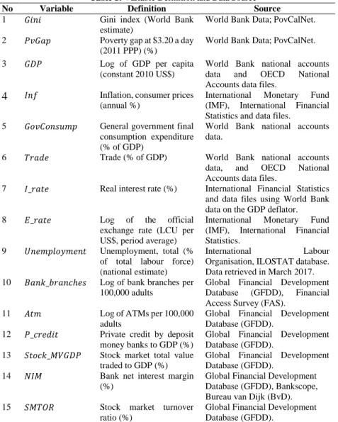
Table 1: Variable Definition and Data Source
No Variable Definition Source
1 𝐺𝑖𝑛𝑖 Gini index (World Bank
estimate)
World Bank Data; PovCalNet.
2 𝑃𝑣𝐺𝑎𝑝 Poverty gap at $3.20 a day (2011 PPP) (%)
World Bank Data; PovCalNet.
3 𝐺𝐷𝑃 Log of GDP per capita
(constant 2010 US$)
World Bank national accounts data and OECD National Accounts data files.
4 𝐼𝑛𝑓 Inflation, consumer prices
(annual %)
International Monetary Fund (IMF), International Financial Statistics and data files.
5 𝐺𝑜𝑣𝐶𝑜𝑛𝑠𝑢𝑚𝑝 General government final consumption expenditure (% of GDP)
World Bank national accounts data.
6 𝑇𝑟𝑎𝑑𝑒 Trade (% of GDP) World Bank national accounts data, and OECD National Accounts data files.
7 𝐼_𝑟𝑎𝑡𝑒 Real interest rate (%) International Financial Statistics and data files using World Bank data on the GDP deflator.
8 𝐸_𝑟𝑎𝑡𝑒 Log of the official exchange rate (LCU per US$, period average)
International Monetary Fund (IMF), International Financial Statistics.
9 𝑈𝑛𝑒𝑚𝑝𝑙𝑜𝑦𝑚𝑒𝑛𝑡 Unemployment, total (%
of total labour force) (national estimate)
International Labour
Organisation, ILOSTAT database.
Data retrieved in March 2017.
10 𝐵𝑎𝑛𝑘_𝑏𝑟𝑎𝑛𝑐ℎ𝑒𝑠 Log of bank branches per 100,000 adults
Global Financial Development Database (GFDD), Financial Access Survey (FAS).
11 𝐴𝑡𝑚 Log of ATMs per 100,000
adults
Global Financial Development Database (GFDD).
12 𝑃_𝑐𝑟𝑒𝑑𝑖𝑡 Private credit by deposit money banks to GDP (%)
Global Financial Development Database (GFDD).
13 𝑆𝑡𝑜𝑐𝑘_𝑀𝑉𝐺𝐷𝑃 Stock market total value traded to GDP (%)
Global Financial Development Database (GFDD).
14 𝑁𝐼𝑀 Bank net interest margin (%)
Global Financial Development Database (GFDD), Bankscope, Bureau van Dijk (BvD).
15 𝑆𝑀𝑇𝑂𝑅 Stock market turnover ratio (%)
Global Financial Development Database (GFDD).
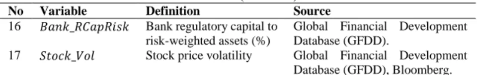
Table 1: (Continue)
No Variable Definition Source
16 𝐵𝑎𝑛𝑘_𝑅𝐶𝑎𝑝𝑅𝑖𝑠𝑘 Bank regulatory capital to risk-weighted assets (%)
Global Financial Development Database (GFDD).
17 𝑆𝑡𝑜𝑐𝑘_𝑉𝑜𝑙 Stock price volatility Global Financial Development Database (GFDD), Bloomberg.
Source: Own elaboration.
4. Results & Discussion
We start our analysis by identifying the output of descriptive statistics. As reflected in the proposed empirical model (model 1 and model 2), we employ each variable which is already transformed (for instance, we do the log transformation for the data of exchange rate, GDP, number of bank branches and the number of ATM). The other variables have been provided in the form of percentage to GDP as documented in the archival data of World Bank Database index and Global Financial Development Database (GFDD).
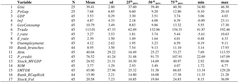
Table 2 presents some fundamental information concerning the number of observations on each variable, mean, standard deviation (sd), 25th percentile, median (50th percentile), 75th percentile, minimum value, and the maximum value of each variable. More precisely, we provide breakdown of our sample by year, by country, and further elaborate the descriptive statistics based on the consolidated sample (Panel A), countries’ mean of inequality, poverty and control variables for each country (Panel B), and the countries’
mean of financial development variables (Panel C). In Panel A, variable Gini as obtained from five ASEAN countries shows an average value of Gini index ratio (mean) as 39.41, where the minimum Gini is 34.8, and the maximum value is 46.3. Here, variable Gini is considered as the proxy of income inequality. Meanwhile, the proxy of the poverty gap is variable PvGap. Variable PvGap provides mean value as 7.68 on average. These two variables are determined as the dependent variables, which quantitatively measure the income inequality and poverty gap among the sample.
Table 2: Descriptive Statistics Panel A. Descriptive statistics of the consolidated data
Variable N Mean sd 25th perc. 50 th perc. 75 th perc. min max
1 𝐺𝑖𝑛𝑖 25 39.41 2.80 37.60 39.40 40.30 34.80 46.30
2 𝑃𝑣𝐺𝑎𝑝 25 7.68 6.85 0.60 9.20 12.80 0.10 20.10
3 𝐺𝐷𝑃 45 3.53 0.29 3.30 3.51 3.74 3.06 4.03
4 𝐼𝑛𝑓 45 4.87 4.33 2.18 4.08 6.39 -0.89 23.11
5 𝐺𝑜𝑣𝐶𝑜𝑛𝑠𝑢𝑚𝑝 45 10.79 3.49 8.83 9.86 13.32 5.55 17.30
6 𝑇𝑟𝑎𝑑𝑒 45 113.01 47.33 62.69 132.06 154.31 41.87 192.46
7 𝐼_𝑟𝑎𝑡𝑒 45 3.27 3.53 1.81 3.74 5.44 -5.61 10.63
8 𝐸_𝑟𝑎𝑡𝑒 45 2.39 1.50 1.49 1.64 4.01 0.48 4.33
9 𝑈𝑛𝑒𝑚𝑝𝑙𝑜𝑦𝑚𝑒𝑛𝑡 45 4.12 2.62 1.95 3.23 6.59 0.19 9.11
10 𝐵𝑎𝑛𝑘_𝑏𝑟𝑎𝑛𝑐ℎ𝑒𝑠 44 8.95 3.50 7.54 9.13 11.10 3.14 17.93
11 𝐴𝑡𝑚 45 40.04 29.22 16.49 25.27 53.27 7.69 113.55
12 𝑃_𝑐𝑟𝑒𝑑𝑖𝑡 45 76.52 41.24 31.48 91.75 107.91 22.69 147.09
13 𝑆𝑡𝑜𝑐𝑘_𝑀𝑉𝐺𝐷𝑃 45 26.92 21.31 10.30 14.69 40.97 2.92 80.06
14 𝑁𝐼𝑀 45 3.77 1.29 2.93 3.49 4.07 1.72 6.77
15 𝑆𝑀𝑇𝑂𝑅 45 45.00 27.96 25.32 31.38 66.65 13.34 129.28
16 𝐵𝑎𝑛𝑘_𝑅𝐶𝑎𝑝𝑅𝑖𝑠𝑘 44 15.90 2.21 14.80 16.08 17.38 11.33 21.28
17 𝑆𝑡𝑜𝑐𝑘_𝑉𝑜𝑙 45 20.58 7.23 16.85 19.84 24.83 8.15 36.09
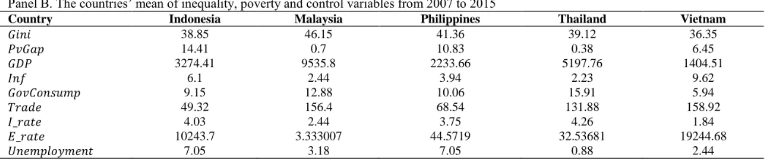
Table 2: (Continue)
Panel B. The countries’ mean of inequality, poverty and control variables from 2007 to 2015
Country Indonesia Malaysia Philippines Thailand Vietnam
𝐺𝑖𝑛𝑖 38.85 46.15 41.36 39.12 36.35
𝑃𝑣𝐺𝑎𝑝 14.41 0.7 10.83 0.38 6.45
𝐺𝐷𝑃 3274.41 9535.8 2233.66 5197.76 1404.51
𝐼𝑛𝑓 6.1 2.44 3.94 2.23 9.62
𝐺𝑜𝑣𝐶𝑜𝑛𝑠𝑢𝑚𝑝 9.15 12.88 10.06 15.91 5.94
𝑇𝑟𝑎𝑑𝑒 49.32 156.4 68.54 131.88 158.92
𝐼_𝑟𝑎𝑡𝑒 4.03 2.44 3.75 4.26 1.84
𝐸_𝑟𝑎𝑡𝑒 10243.7 3.333007 44.5719 32.53681 19244.68
𝑈𝑛𝑒𝑚𝑝𝑙𝑜𝑦𝑚𝑒𝑛𝑡 7.05 3.18 7.05 0.88 2.44
Panel C. The countries’ mean of financial development dimensions from 2007 to 2015
Country Indonesia Malaysia Philippines Thailand Vietnam
𝐵𝑎𝑛𝑘_𝑏𝑟𝑎𝑛𝑐ℎ𝑒𝑠 10.25 11.02 7.97 11.40 3.49
𝐴𝑡𝑚 27.68 49.88 17.95 86.74 17.96
𝑃_𝑐𝑟𝑒𝑑𝑖𝑡 28.49 106.66 31.21 125.73 90.52
𝑆𝑡𝑜𝑐𝑘_𝑀𝑉𝐺𝐷𝑃 12.35 43.85 11.89 57.22 9.30
𝑁𝐼𝑀 6.01 2.64 3.73 3.16 3.33
𝑆𝑀𝑇𝑂𝑅 35.35 33.35 18.82 79.05 58.41
𝐵𝑎𝑛𝑘_𝑅𝐶𝑎𝑝𝑅𝑖𝑠𝑘 18.32 16.456 16.23 15.62 12.52
𝑆𝑡𝑜𝑐𝑘_𝑉𝑜𝑙 22.81 11.99 21.18 21.64 25.29
Data source: World Bank Database and the Global Financial Development Database, for years 2007-2015. See Table 1 for variable definitions and scales.
Notes: Table 2 reports the information regarding the information of descriptive statistics of the variables and several country-effect data obtained from the macroeconomic variables.
Moreover, this study employs several control variables regarding the effort of neutralising the confounding effects that resulted from the interaction between the main variable. The control variables are originally identified from the previous works of literature on the finance-inequality- poverty links. Hereby, macroeconomics variables are utilised. The mean of variable GDP per capita is noted as 3.53 ($ 4,329) on average, followed by variable Inf as 4.87% on average. Variable GovConsump reports mean value as 10.79. Variable Trade further shows a mean value as 113.01 on average.
I_rate as which is the interest rate shows mean value as 3.27% on average.
Variable E_rate denotes as the exchange rate value which has been transformed into log data and notes the mean value as 2.394 (5,913 compared with the U.S. Dollar) on average. The last control variable is the level of the Unemployment rate, where the data of five ASEAN countries (Indonesia, Malaysia, Philippines, Thailand, and Vietnam) reports 4.12% unemployment on average.
The main independent variable is financial development (FD), which is proxied by four financial dimensions; First, financial access, which is surrogated by Bank_branches and the number of ATMs. Second, financial deepening, which is proxied by P_credit and Stock_MVGDP. Third, financial efficiency is surrogated by NIM and SMTOR. Fourth, financial stability is represented by the usage of variable Bank_RCapRisk and Stock_Vol. All of these four dimensions are the measures of Financial Development (FD) that is conjectured to be associated with income inequality (Gini) and Poverty (PvGap).
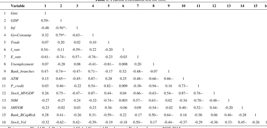
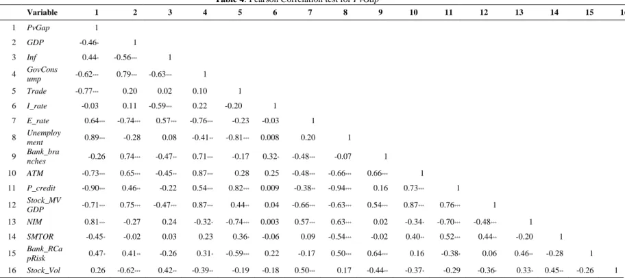
Table 3 provides the correlation output between the main independent variable, control variable and Gini as the main dependent variable. Table 4 also presents the correlation output of each independent and control variable with PvGap as the dependent variable. The aim of separating the correlation output is due to the different usage of the dependent variable. Also, in this respect, we would like to differentiate the effect of financial development on two different measures of income inequality and poverty gap. The information in Tables 3 and 4 depicts the correlation among the variables. It is documented that most of the variable of financial development is strongly correlated with poverty (PvGap) rather than to income inequality (Gini).
Therefore, further investigation needs to be conducted in terms of causal- effect test from the financial development dimensions (Financial access;
(Bank_Branches and ATM), financial deepening; (P_credit and Stock_MVGDP), financial efficiency; (NIM and SMTOR) and financial stability; (Bank_RCapRisk and Stock_Vol) to variable income inequality (Gini) and poverty (PvGap).
Table 3: Pearson Correlation test for Gini
Variable 1 2 3 4 5 6 7 8 9 10 11 12 13 14 15 16
1 Gini 1
2 GDP 0.59** 1
3 Inf -0.48* -0.56*** 1
4 GovConsump 0.32 0.79*** -0.63*** 1
5 Trade 0.07 0.20 0.02 0.10 1
6 I_rate 0.54** 0.11 -0.59*** 0.22 -0.20 1 7 E_rate -0.61** -0.74*** 0.57*** -0.76*** -0.23 -0.03 1
8 Unemployment 0.07 -0.28 0.08 -0.41** -0.81*** 0.008 0.20 1 9 Bank_branches 0.47* 0.74*** -0.47** 0.71*** -0.17 0.32* -0.48*** -0.07 1 10 ATM 0.15 0.65*** -0.45** 0.87*** 0.28 0.25 -0.48*** -0.66*** 0.66*** 1 11 P_credit 0.03 0.46** -0.22 0.54*** 0.82*** 0.009 -0.38** -0.94*** 0.16 0.73*** 1
12 Stock_MVGDP 0.26 0.75*** -0.47*** 0.87*** 0.44** 0.04 -0.66*** -0.63*** 0.54*** 0.87*** 0.76*** 1 13 NIM -0.27 -0.27 0.24 -0.32* -0.74*** 0.003 0.57*** 0.63*** 0.02 -0.34* -0.70*** -0.48*** 1 14 SMTOR -0.23 -0.02 0.03 0.23 0.36* -0.06 0.09 -0.54*** -0.02 0.40** 0.52*** 0.44** -0.20 1 15 Bank_RCapRisk 0.28 0.41** -0.26 0.31* -0.59*** 0.22 -0.17 0.50*** 0.64*** 0.16 -0.38* 0.06 0.46** -0.28 1 16 Stock_Vol -0.32 -0.62*** 0.42** -0.39** -0.19 -0.18 0.50*** 0.17 -0.44** -0.37* -0.29 -0.36* 0.33* 0.45** -0.26 1
Data source: World Bank Database and Global Financial Development Database, for years 2007-2015.
See Table. 1 for the definition of variables. Table 5 displays Pearson correlation coefficients among the employed variables. Each asterisk indicates statistical significance where; *** p<0.01, ** p<0.05, and * p<0.1 respectively using two-tail test.
Table 4: Pearson Correlation test for PvGap
Variable 1 2 3 4 5 6 7 8 9 10 11 12 13 14 15 16
1 PvGap 1
2 GDP -0.46* 1
3 Inf 0.44* -0.56*** 1
4 GovCons
ump -0.62*** 0.79*** -0.63*** 1
5 Trade -0.77*** 0.20 0.02 0.10 1
6 I_rate -0.03 0.11 -0.59*** 0.22 -0.20 1
7 E_rate 0.64*** -0.74*** 0.57*** -0.76*** -0.23 -0.03 1 8 Unemploy
ment 0.89*** -0.28 0.08 -0.41** -0.81*** 0.008 0.20 1 9 Bank_bra
nches -0.26 0.74*** -0.47** 0.71*** -0.17 0.32* -0.48*** -0.07 1
10 ATM -0.73*** 0.65*** -0.45** 0.87*** 0.28 0.25 -0.48*** -0.66*** 0.66*** 1
11 P_credit -0.90*** 0.46** -0.22 0.54*** 0.82*** 0.009 -0.38** -0.94*** 0.16 0.73*** 1 12 Stock_MV
GDP -0.71*** 0.75*** -0.47*** 0.87*** 0.44** 0.04 -0.66*** -0.63*** 0.54*** 0.87*** 0.76*** 1
13 NIM 0.81*** -0.27 0.24 -0.32* -0.74*** 0.003 0.57*** 0.63*** 0.02 -0.34* -0.70*** -0.48*** 1 14 SMTOR -0.45* -0.02 0.03 0.23 0.36* -0.06 0.09 -0.54*** -0.02 0.40** 0.52*** 0.44** -0.20 1 15 Bank_RCa
pRisk 0.47* 0.41** -0.26 0.31* -0.59*** 0.22 -0.17 0.50*** 0.64*** 0.16 -0.38* 0.06 0.46** -0.28 1 16 Stock_Vol 0.26 -0.62*** 0.42** -0.39** -0.19 -0.18 0.50*** 0.17 -0.44** -0.37* -0.29 -0.36* 0.33* 0.45** -0.26 1
Data source: Worldbank database and Global Financial Development Database, for years 2007-2015.
See Table. 1 for the definition of variables. Table 5 displays Pearson correlation coefficients among the employed variables. Each asterisk indicates statistical significance where; *** p<0.01, ** p<0.05, and * p<0.1 respectively using two-tail test.
If we compare the result of correlation test between the link of financial development-inequality and financial development-poverty, it can be reported that financial development has shown stronger correlation and statistically more significant to poverty than to income inequality. With this, the information in Table 2 shows that only one proxy of financial development (financial access: Bank_branches), which shows positive and statistically correlated to income inequality that is proxied by Gini. However, on the other hand, most of all the four dimensions of financial development (financial access, financial deepening, financial efficiency, and financial stability) have performed significant correlation with poverty (PvGap).
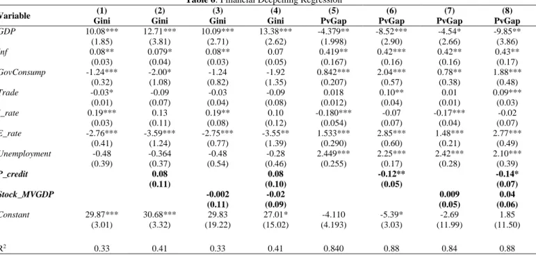
After elaborating on the correlation test (Pearson correlation test) among the main independent and dependent variables, we continue with hypotheses testing. We recognise that our data is classified as the unbalanced data, which use the four financial dimensions with at least two parameters as the surrogate indicators of each dimension. Therefore, we do the hierarchical panel data regression analysis on the different proposed model (model 1 and model 2). We first test the effect of financial access as the proxy of financial development by using two surrogate indicators as Bank_branches and ATM.
The complete output of hierarchical unbalanced panel data analysis is provided as follows.
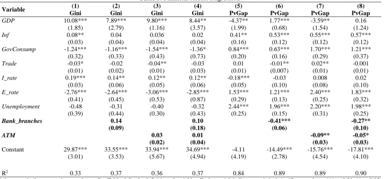
As seen in Table 5, the first dimension of variable financial development, which is tested through the proposed empirical model is financial access. The surrogate indicators to empirically test the financial access are the variable Bank_branches and ATM. These two variables represent the financial access ability, which is conjectured to be associated with income inequality (Gini) and poverty (PvGap). We employ the following statistical models to run the regression. The first model is to see the impact of financial access on Gini where;
𝐺𝑖𝑛𝑖𝑖,𝑡 = 𝛼 + 𝜷𝑩𝒂𝒏𝒌𝒃𝒓𝒂𝒏𝒄𝒉𝒆𝒔𝒊,𝒕+ 𝜷𝑨𝒕𝒎𝒊,𝒕+ 𝛾1𝐺𝐷𝑃𝑖,𝑡+ 𝛾2𝐼𝑛𝑓𝑖,𝑡 + 𝛾3𝐺𝑜𝑣𝐶𝑜𝑛𝑠𝑢𝑚𝑝𝑖,𝑡+ 𝛾4𝑇𝑟𝑎𝑑𝑒𝑖,𝑡+ 𝛾5𝐼𝑟𝑎𝑡𝑒𝑖,𝑡
+ 𝛾6𝐸_𝑟𝑎𝑡𝑒𝑖,𝑡+ 𝛾7𝑈𝑛𝑒𝑚𝑝𝑙𝑜𝑦𝑚𝑒𝑛𝑡𝑖,𝑡+ 𝜀𝑖,𝑡
In the second model, we test the impact of financial access on the poverty gap where;
𝑃𝑣𝐺𝑎𝑝𝑖,𝑡 = 𝛼 + 𝜷𝑩𝒂𝒏𝒌𝒃𝒓𝒂𝒏𝒄𝒉𝒆𝒔𝒊,𝒕+ 𝜷𝑨𝒕𝒎𝒊,𝒕+ 𝛾1𝐺𝐷𝑃𝑖,𝑡+ 𝛾2𝐼𝑛𝑓𝑖,𝑡 + 𝛾3𝐺𝑜𝑣𝐶𝑜𝑛𝑠𝑢𝑚𝑝𝑖,𝑡+ 𝛾4𝑇𝑟𝑎𝑑𝑒𝑖,𝑡+ 𝛾5𝐼𝑟𝑎𝑡𝑒𝑖,𝑡
+ 𝛾6𝐸_𝑟𝑎𝑡𝑒𝑖,𝑡+ 𝛾7𝑈𝑛𝑒𝑚𝑝𝑙𝑜𝑦𝑚𝑒𝑛𝑡𝑖,𝑡+ 𝜀𝑖,𝑡
Table 5: Financial Access Regression
Variable (1) (2) (3) (4) (5) (6) (7) (8)
Gini Gini Gini Gini PvGap PvGap PvGap PvGap
GDP 10.08*** 7.89*** 9.80*** 8.44** -4.37** 1.77*** -3.59** 0.16
(1.85) (2.79) (1.16) (3.57) (1.99) (0.68) (1.54) (1.24)
Inf 0.08** 0.04 0.036 0.02 0.41** 0.53*** 0.55*** 0.57***
(0.03) (0.04) (0.04) (0.04) (0.16) (0.12) (0.12) (0.12)
GovConsump -1.24*** -1.16*** -1.54*** -1.36* 0.84*** 0.63*** 1.70*** 1.21***
(0.32) (0.33) (0.43) (0.73) (0.20) (0.16) (0.29) (0.37)
Trade -0.03* -0.02 -0.04** -0.03 0.01 -0.01** 0.02** -0.001
(0.01) (0.02) (0.01) (0.03) (0.01) (0.007) (0.01) (0.01)
I_rate 0.19*** 0.14** 0.12** 0.12** -0.18*** -0.03 0.008 0.02
(0.03) (0.06) (0.05) (0.06) (0.05) (0.10) (0.08) (0.10)
E_rate -2.76*** -2.64*** -3.06*** -2.85*** 1.53*** 1.21*** 2.40*** 1.83***
(0.41) (0.45) (0.53) (0.87) (0.29) (0.13) (0.25) (0.32)
Unemployment -0.48 -0.31 -0.40 -0.32 2.44*** 1.96*** 2.20*** 1.98***
(0.39) (0.44) (0.30) (0.43) (0.25) (0.15) (0.31) (0.25)
Bank_branches 0.14 0.10 -0.41*** -0.27**
(0.09) (0.18) (0.06) (0.10)
ATM 0.03 0.01 -0.09** -0.05*
(0.02) (0.04) (0.03) (0.03)
Constant 29.87*** 33.55*** 33.94*** 34.69*** -4.11 -14.49*** -15.76*** -17.81***
(3.01) (3.53) (5.67) (4.94) (4.19) (2.78) (4.54) (4.10)
R2 0.33 0.37 0.36 0.37 0.84 0.89 0.89 0.90
Robust standard errors are in parentheses. See Table. 1 for the definition of variables. Each asterisk indicates statistical significance where; *** p<0.01, ** p<0.05,
* p<0.1 respectively using a two-tail test.
Notes: In the un-tabulated results of 2SLS with instrumental variable (IV), the usage of the lagged variable for the financial access dimension results in consistent output by employing the contemporaneous variable as seen in Table 5. In this case, the lagged variables of Bank_branches t-1 and ATM t-1 have performed no significant association with the income inequality (Gini), and remain consistent in the association of financial access with poverty (p< 0.01).