DECISION MAKING – THE ANALYTIC HIERARCHY AND NETWORK PROCESSES (AHP/ANP)
Thomas L. SAATY
University of Pittsburgh [email protected] Abstract
This is the first part of an introduction to multicriteria decision making using the Analytic Hierarchy Process (AHP) and its generalization, the Analytic Network Process (ANP). The discussion involves individual and group decisions both with the independence of the criteria from the alternatives as in the AHP and also with dependence and feedback in the entire decision structure as in the ANP. This part explains the Analytic Hierarchy Process, with examples, and presents in some detail the mathematical foundations. An exposition of the Analytic Network Process and its applications will appear in later issues of this journal.
Keywords: Decision making, Analytic Hierarchy Process (AHP), Analytic Network Process (ANP)
1. Introduction
(Saaty 1977, 1994, 2000a, 2000b and 2001)Decision making involves criteria and alternatives to choose from. The criteria usually have different importance and the alternatives in turn differ in our preference for them on each criterion. To make such tradeoffs and choices we need a way to measure.
Measuring needs a good understanding of methods of measurement and different scales of measurement.
Many people think that measurement needs a physical scale with a zero and a unit to apply to objects or phenomena. That is not true.
Surprisingly enough, we can also derive accurate and reliable relative scales that do not have a zero or a unit by using our understanding and judgments that are, after all,
the most fundamental determinants of why we want to measure something. In reality we do that all the time and we do it subconsciously without thinking about it. Physical scales help our understanding and use of the things that we know how to measure. After we obtain readings from a physical scale, they still need to be interpreted according to what they mean and how adequate or inadequate they are to satisfy some need we have. But the number of things we don’t know how to measure is infinitely larger than the things we know how to measure, and it is highly unlikely that we will ever find ways to measure everything on a physical scale with a unit. Scales of measurement are inventions of a technological mind. Our minds and ways of understanding we have had with us and will always have. The brain is an electrical device of neurons whose
firings and synthesis must perform measurement with great accuracy to give us all the meaning and understanding that we have to enable us to survive and reach out to control a complex world. Can we rely on our minds to be accurate guides with their judgments? The answer depends on how well we know the phenomena to which we apply measurement and how good our judgments are to represent our understanding. In our own personal affairs we are the best judges of what may be good for us. In situations involving many people, we need the judgments from all the participants. In general we think that there are people who are more expert than others in some areas and their judgments should have precedence over the judgments of those who know less as in fact is often the case in practice.
Judgments expressed in the form of comparisons are fundamental in our biological makeup. They are intrinsic in the operations of our brains and that of animals and one might even say of plants since, for example, they control how much sunlight to admit. We all make decisions every moment, consciously or unconsciously, today and tomorrow, now and forever, it seems. Decision-making is a fundamental process that is integral in everything we do. How do we do it? The Harvard psychologist Arthur Blumenthal tells us in his book The Process of Cognition, Prentice-Hall, Inc., Englewood Cliffs, New Jersey, 1977, that there are two types of judgment: “Comparative judgment which is the identification of some relation between two stimuli both present to the observer, and absolute judgment which involves the relation between a single stimulus and some
information held in short term memory about some former comparison stimuli or about some previously experienced measurement scale using which the observer rates the single stimulus.”
When we think about it, both these processes involve making comparisons.
Comparisons imply that all things we know are understood in relative terms to other things. It does not seem possible to know an absolute in itself independently of something else that influences it or that it influences. The question then is how do we make comparisons in a scientific way and derive from these comparisons scales of relative measurement?
When we have many scales with respect to a diversity of criteria and subcriteria, how do we synthesize these scales to obtain an overall relative scale? Can we validate this process so that we can trust its reliability? What can we say about other ways people have proposed to deal with judgment and measurement, how do they relate to this fundamental idea of comparisons, and can they be relied on for validity? These are all questions we need to consider in making a decision. It is useful to remember that there are many people in the world who only know their feelings and may know nothing about numbers and never heard of them but can still make good decisions, how do they do it? It is unlikely that by guessing at numbers and assigning them directly to the alternatives to indicate order under a criterion will yield meaningful priorities because the numbers are arbitrary. Even if they are taken from a scale for a particular criterion, how would we combine them across the criteria as they would likely be from different scales? Our answer to this conundrum is to derive a relative
scale for the criteria with respect to the goal and to derive relative scales for the alternatives with respect to each of the criteria and use a weighting and adding process that will make these scales alike. The scale we derive under each criterion is the same priority scale that measures the preference we have for the alternatives with respect to each criterion, and the importance we attribute to the criteria in terms of the goal. As we shall see below, the judgments made use absolute numbers and the priorities derived from them are also absolute numbers that represent relative dominance.
Among the many applications made by companies and governments, now perhaps numbering in the thousands, the Analytic Hierarchy Process was used by IBM as part of its quality improvement strategy to design its AS/400 computer and win the prestigious Malcolm Baldrige National Quality Award (Bauer et al. 1992).
2. Deriving a Scale of Priorities from Pairwise Comparisons
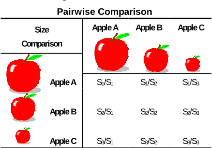
Suppose we wish to derive a scale of relative importance according to size (volume) of three apples A, B, C shown in Figure 1.
Assume that their volumes are known respectively as S S1, 2 and S3. For each position in the matrix the volume of the apple at the left is compared with that of the apple at the top and the ratio is entered. A matrix of judgmentsA=(aij)is constructed with respect to a particular property the elements have in common. It is reciprocal, that is,aji =1/aij, and aii =1. For the matrix in Figure 1, it is necessary to make only three judgments with the remainder being automatically determined.
There are n n( −1) / 2 judgments required for a matrix of ordern. Sometimes one (particularly an expert who knows well what the judgments should be) may wish to make a minimum set of judgments and construct a consistent matrix defined as one whose entries satisfy
ij jk ik
a a =a , i j k, , =1,L,n . To do this one can enter n−1 judgments in a row or in a column, or in a spanning set with at least one judgment in every row and column, and construct the rest of the entries in the matrix using the consistency condition. Redundancy in the number of judgments generally improves the validity of the final answer because the judgments of the few elements one chooses to compare may be more biased.
Pairwise Comparison
Apple A Apple B Apple C Size
Comparison
Apple A S1/S1 S1/S2 S1/S3
Apple B S2/S1 S2/S2 S2/S3
Apple C S3/S1 S3/S2 S3/S3
Figure 1 Reciprocal structure of pairwise comparison matrix for apples
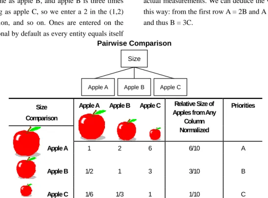
Assume that we know the volumes of the apples so that the values we enter in Figure 2 are consistent. Apple A is twice as big in volume as apple B, and apple B is three times as big as apple C, so we enter a 2 in the (1,2) position, and so on. Ones are entered on the diagonal by default as every entity equals itself
on any criterion. Note that in the (2, 3) position we can enter the value 3 because we know the judgments are consistent as they are based on actual measurements. We can deduce the value this way: from the first row A = 2B and A = 6C, and thus B = 3C.
Pairwise Comparison Size
Apple B Apple C Apple A
Apple A Apple B Apple C Size
Comparison
Relative Size of Apples from Any
Column Normalized
Priorities
Apple A 1 2 6 6/10 A
Apple B 1/2 1 3 3/10 B
Apple C 1/6 1/3 1 1/10 C
Figure 2 Pairwise comparison matrix for apples using judgments If we did not have actual measurements, we
could not be certain that the judgments in the first row are accurate, and we would not mind estimating the value in the (2, 3) position directly by comparing apple B with apple C.
We are then very likely to be inconsistent. How inconsistent can we be before we think it is intolerable? Later we give an actual measure of inconsistency and argue that a consistency of about 10% is considered acceptable.
We obtain from the consistent pairwise comparison matrix above a vector of priorities showing the relative sizes of the apples. Note that we do not have to go to all this trouble to derive the relative volumes of the apples. We
could simply have normalized the actual measurements. The reason we did so is to lay the foundation for what to do when we have no measures for the property in question. When judgments are consistent as they are here, this vector of priorities can be obtained in two ways: dividing the elements in any column by the sum of its entries (normalizing it), or by summing the entries in each row to obtain the overall dominance in size of that alternative relative to the others and normalizing the resulting column of values. Incidentally, calculating dominance plays an important role in computing the priorities when judgments are inconsistent for then an alternative may
dominate another by different magnitudes by transiting to it through intermediate alternatives. Thus the story is very different if the judgments are inconsistent, and we need to allow inconsistent judgments for good reasons.
In sports, team A beats team B, team B beats team C, but team C beats team A. How would we admit such an occurrence in our attempt to explain the real world if we do not allow inconsistency? Most theories have taken a stand against such an occurrence with an axiom that assumes transitivity and prohibits intransitivity, although one does not have to be intransitive to be inconsistent in the values obtained. Others have wished it away by saying that it should not happen in human thinking. But it does, and we offer a theory below that copes with intransitivity.
3. The Fundamental Scale of the AHP for Making
Comparisons with Judgments
If we were to use judgments instead of ratios, we would estimate the ratios as numbers using the Fundamental Scale of the AHP, shown in Table 1 and derived analytically later in the paper, and enter these judgments in the matrix. A judgment is made on a pair of elements with respect to a property they have in common. The smaller element is considered to be the unit and one estimates how many times more important, preferable or likely, more generally “dominant”, the other is by using a number from the Fundamental Scale.
Dominance is often interpreted as importance when comparing the criteria and as preference
when comparing the alternatives with respect to the criteria. It can also be interpreted as likelihood as in the likelihood of a person getting elected as president, or other terms that fit the situation.
The set of objects being pairwise compared must be homogeneous. That is, the dominance of the largest object must be no more than 9 times the smallest one (this is the widest span we use for many good reasons discussed elsewhere in the AHP literature). Things that differ by more than this range can be clustered into homogeneous groups and dealt with by using this scale. If measurements from an existing scale are used, they can simply be normalized without regard to homogeneity.
When the elements being compared are very close, they should be compared with other more contrasting elements, and the larger of the two should be favored a little in the judgments over the smaller. We have found this approach to be effective to bring out the actual priorities of the two close elements.
Otherwise we have proposed the use of a scale between 1 and 2 using decimals and similar judgments to the Fundamental Scale below. We note that human judgment is relatively insensitive to such small decimal changes.
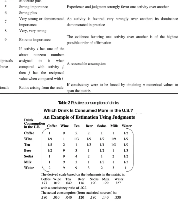
Table 2 shows how an audience of about 30 people, using consensus to arrive at each judgment, provided judgments to estimate the dominance of the consumption of drinks in the United States (which drink is consumed more in the US and how much more than another drink?). The derived vector of relative consumption and the actual vector, obtained by normalizing the consumption given in official statistical data sources, are at the bottom of the table.
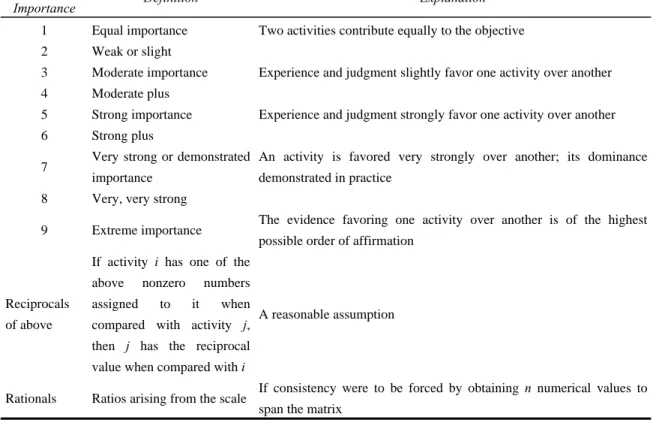
Table 1 The Fundamental scale of absolute numbers Intensity of
Importance Definition Explanation
1 Equal importance Two activities contribute equally to the objective 2 Weak or slight
3 Moderate importance Experience and judgment slightly favor one activity over another 4 Moderate plus
5 Strong importance Experience and judgment strongly favor one activity over another 6 Strong plus
7 Very strong or demonstrated importance
An activity is favored very strongly over another; its dominance demonstrated in practice
8 Very, very strong
9 Extreme importance The evidence favoring one activity over another is of the highest possible order of affirmation
Reciprocals of above
If activity i has one of the above nonzero numbers assigned to it when compared with activity j, then j has the reciprocal value when compared with i
A reasonable assumption
Rationals Ratios arising from the scale If consistency were to be forced by obtaining n numerical values to span the matrix
Table 2 Relative consumption of drinks
Which Drink Is Consumed More in the U.S.?
W c s Co su ed o e e U.S.?
An Example of Estimation Using Judgments
Coffee Wine Tea Beer Sodas Milk Water Drink
Consumption in the U.S.
Coffee Wine Tea Beer Sodas Milk Water
1 1/9 1/5 1/2 1 1 2
9 1 2 9 9 9 9
5 1/3
1 3 4 3 9
2 1/9 1/3 1 2 1 3
1 1/9 1/4 1/2 1 1/2
2 1 1/9 1/3 1 2 1 3
1/2 1/9 1/9 1/3 1/2 1/3 1 The derived scale based on the judgments in the matrix is:
Coffee Wine Tea Beer Sodas Milk Water .177 .019 .042 .116 .190 .129 .327 with a consistency ratio of .022.
The actual consumption (from statistical sources) is:
.180 .010 .040 .120 .180 .140 .330
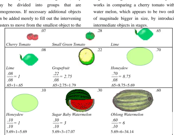
If the objects are not homogeneous, they may be divided into groups that are homogeneous. If necessary additional objects can be added merely to fill out the intervening clusters to move from the smallest object to the
largest one. Figure 3 shows how this process works in comparing a cherry tomato with a water melon, which appears to be two orders of magnitude bigger in size, by introducing intermediate objects in stages.
Figure 3 Clustering to compare non-homogeneous objects
4. Scales of Measurement
Mathematically a scale is a triple, a set of numbers, a set of objects and a mapping of the objects to the numbers. There are two ways to perform measurement, one is by using an instrument and making the correspondence directly, and the other is by using judgment.
When using judgments one can either assign numbers to the objects by guessing their value on some scale of measurement when there is one, or derive a scale by considering a subset of objects in some fashion such as comparing them in pairs, thus making the correspondence
indirect. In addition there are two kinds of origin; one is an absolute origin as in absolute temperature where nothing falls below that reading; and the other where the origin is a dividing point of positive and negative values with no bound on either side such as with a thermometer. Underlying both these ways are the following kinds (there can be more) of general scales:
Nominal Scale invariant under one to one correspondence where a number is assigned to each object; for example, handing out numbers for order of service to people in a queue.
Ordinal Scale invariant under monotone
.07 .28 .65
Cherry Tomato Small Green Tomato Lime
.08 .22 .70
Lime .08= 1 .08 .65×1=.65
Grapefruit .22= 2.75 .08
.65×2.75=1.79
Honeydew .70= 8.75 .08
.65×8.75=5.69
.10 .30 .60
Honeydew .10= 1 .10 5.69×1=5.69
Sugar Baby Watermelon .30= 3
.10
5.69×3=17.07
Oblong Watermelon .60= 6
.10
5.69×6=34.14 This means that 34.14/.07.487.7 cherry tomatoes are equal to the oblong watermelon.
transformations, where things are ordered by number but the magnitudes of the numbers only serve to designate order, increasing or decreasing; for example, assigning two numbers 1 and 2, to two people to indicate that one is taller than the other, without including any information about their actual heights. The smaller number may be assigned to the taller person and vice versa.
Interval Scale invariant under a positive linear transformation; for example, the linear transformation F = (9/5) C + 32 for converting a Celsius to a Fahrenheit temperature reading.
Note that one cannot add two readings
x
1 andx
2 on an interval scale because then1+ 2 ( + ) 1 ( 2 ) ( 1 )2
y y = a x b + a x + b =a x + x 2 b
+ which is of the form ax+2 b and not of the form ax b+ . However, one can take an average of such readings because dividing by 2 yields the correct form.
Ratio Scale invariant under a similarity transformation, y ax= , a>0. An example is converting weight measured in pounds to kilograms by using the similarity transformation K = 2.2 P. The ratio of the weights of the two objects is the same regardless of whether the measurements are done in pounds or in kilograms. Zero is not the measurement of anything; it applies to objects that do not have the property and in addition one cannot divide by zero to preserve ratios in a meaningful way. Note that one can add two readings from a ratio scale, but not multiply them because a x x2 1 2 does not have the form ax. The ratio of two readings from a ratio scale such as 6 kg/ 3 kg = 2 is a number that belongs to an absolute scale that says that the 6 kg object is twice heavier than the 3 kg object.
The ratio 2 cannot be changed by some formula to another number. Thus we introduce the next scale.
Absolute Scale invariant under the identity transformation x = x; for example, numbers used in counting the people in a room.
There are also other less well-known scales like a logarithmic and a log-normal scale.
The fundamental scale of the AHP is a scale of absolute numbers used to answer the basic question in all pairwise comparisons:
how many times more dominant is one element than the other with respect to a certain criterion or attribute? The derived scale, obtained by solving a system of homogeneous linear equations whose coefficients are absolute numbers, is also an absolute scale of relative numbers. Such a relative scale does not have a unit nor does it have an absolute zero. The derived scale is like probabilities in not having a unit or an absolute zero.
In a judgment matrix A , instead of assigning two numbers wi and wj (that generally we do not know), as one does with tangibles, and forming the ratio w wi/ j we assign a single number drawn from the fundamental scale of absolute numbers shown in Table 1 above to represent the ratio
(w wi/ j) /1 . It is a nearest integer approximation to the ratio w wi/ j. The ratio of two numbers from a ratio scale (invariant under multiplication by a positive constant) is an absolute number (invariant under the identity transformation) and is dimensionless.
In other words it is not measured on a scale with a unit starting from zero. The numbers of an absolute scale are defined in terms of
similarity or equivalence. The (absolute) number of a class is the class of all those classes that are similar to it; that is they can be put into one-to-one correspondence with it. But that is not our complete story about absolute numbers transformed to relative form – relative absolute numbers. We now continue our account.
The derived scale will reveal what wiand wj are. This is a central fact about the relative measurement approach. It needs a fundamental scale to express numerically the relative dominance relationship by using the smaller or lesser element as the unit of each comparison.
Some people who do not understand this and regard the AHP as controversial, forget that most people in the world don’t think in terms of numbers but of how they feel about intensities of dominance. They think that the AHP would have a greater theoretical strength if the judgments were made in terms of “ratios of preference differences”. I think that the layman would find this proposal laughable as I do for its paucity of understanding, taking the difference of non-existing numbers which one is trying to find in the first place. He needs first to see a utility doctor who would help him create an interval scale utility function so he can take values from it to form differences and then form their ratios to get one judgment!
5. From Consistency to Inconsistency
Consistency is essential in human thinking because it enables us to order the world according to dominance. It is a necessary
condition for thinking about the world in a scientific way, but it is not sufficient because a mentally disturbed person can think in a perfectly consistent way about a world that does not exist. We need actual knowledge about the world to validate our thinking. But if we were always consistent we would not be able to change our minds. New knowledge often requires that we see things in a new light that can contradict what we thought was correct before. Thus we live with the contradiction that we must be consistent to capture valid knowledge about the world but at the same time be ready to change our minds and be inconsistent if new information requires that we think differently than we thought before. It is clear that large inconsistency unsettles our thinking and thus we need to change our minds in small steps to integrate new information in the old total scheme. This means that inconsistency must be large enough to allow for change in our consistent understanding but small enough to make it possible to adapt our old beliefs to new information. This means that inconsistency must be precisely one order of magnitude less important than consistency, or simply 10% of the total concern with consistent measurement.
If it were larger it would disrupt consistent measurement and if it were smaller it would make insignificant contribution to change in measurement.
The paired comparisons process using actual measurements for the elements being compared leads to the following consistent reciprocal matrix:
1 2
1 2
1 1 1 1 2 1
2 2 1 2 2 2
1 2
n n
n n
n n n n n
A A A
w w w
A w w w w w w
A w w w w w w
A w w w w w w
L L L L
M M
L
We note that we can recover the vector
(
1,...,
n)
w = w w
by solving the system of equations defined by:1 2
2 2 2 2
2
2 2
1 1 1 n
1 n
n 1 n n n
1 1
n n
w w w w w w
w w w w w w
Aw
w w w w w w
w w
w n w nw
w w
=
⋅ = =
K K M K
M M
Solving this homogeneous system of linear equations Aw nw= to find w is a trivial eigenvalue problem, because the existence of a solution depends on whether or not n is an eigenvalue of the characteristic equation of A.
But A has rank one and thus all its eigenvalues but one are equal to zero. The sum of the eigenvalues of a matrix is equal to its trace, the sum of its diagonal elements, which in this case is equal to n. Thus n is the largest or the principal eigenvalue of A and w is its corresponding principal eigenvector that is positive and unique to within multiplication by a constant, and thus belongs to a ratio scale.
We now know what must be done to recover the weightswi , whether they are known in advance or not.
We said earlier that an n by n matrix ( ij)
A= a is consistent if a aij jk =aik, , , 1,...,
i j k= n holds among its entries. We have for a consistent matrix Ak =nk−1A, a constant times the original matrix. In normalized form both A and Ak have the same principal eigenvector. That is not so for an inconsistent matrix. A consistent matrix always has the form
i j
A w w
=
.
Of course, real-world pairwise comparison matrices are very unlikely to be consistent.
In the inconsistent case, the normalized sum of the rows of each power of the matrix contributes to the final priority vector. Using Cesaro summability and the well-known theorem of Perron, we are led to derive the priorities in the form of the principal right eigenvector. Now we give an elegant mathematical discussion, based on the concept of invariance, to show why we still need for an inconsistent matrix the principal right eigenvector for our priority vector. It is clear that no matter what method we use to derive the weightswi, we need to get them back as proportional to the expression
1
1,...,
n ij j
j a w i n
= =
∑ ,
that is, we must solve
1
= 1,...,
n
ij j i
j a w cw i n
= =
∑ .
Otherwise
1
1,...,
n ij j j
a w i n
= =
∑
would yield another set of different weights
and they in turn can be used to form new expressions
1
1,...,
n ij j
j a w i n
= =
∑ ,
and so on ad infinitum. Unless we solve the principal eigenvalue problem, our quest for priorities becomes meaningless.
We learn from the consistent case that what we get on the right is proportional to the sum on the left that involves the same ratio scale used to weight the judgments that we are looking for. Thus we have the proportionality constant c. A better way to see this is to use the derived vector of priorities to weight each row of the matrix and take the sum. This yields a new vector of priorities (relative dominance of each element) represented in the comparisons.
This vector can again be used to weight the rows and obtain still another vector of priorities. In the limit (if one exists), the limit vector itself can be used to weight the rows and get the limit vector back perhaps proportionately. Our general problem possibly with inconsistent judgments takes the form:
12 1 1
12 2 2
1 2
1 ...
1/ 1 ...
1/ 1/ ... 1
n n
n n n
a a w
a a w
Aw cw
a a w
= =
M M
This homogeneous system of linear equations Aw cw= has a solution w if c is the principal eigenvalue of A. That this is the case can be shown using an argument that involves both left and right eigenvectors of A.
Two vectors x=( ,...,x1 xn), (y= y1,...,yn)are orthogonal if their scalar product
1 1 ... n n
x y + +x y is equal to zero. It is known that any left eigenvector of a matrix corresponding to an eigenvalue is orthogonal to any right eigenvector corresponding to a different eigenvalue. This property is known as biorthogonality (Horn and Johnson 1985).
Theorem For a given positive matrix A, the only positive vector w and only positive constant c that satisfy Aw cw= , is a vector w that is a positive multiple of the principal eigenvector of A, and the only such c is the principal eigenvalue of A.
Proof. We know that the right principal eigenvector and the principal eigenvalue satisfy our requirements. We also know that the algebraic multiplicity of the principal eigenvalue is one, and that there is a positive left eigenvector of A (call it z) corresponding to the principal eigenvalue. Suppose there is a positive vector y and a (necessarily positive) scalar d such thatAy dy= . If d and c are not equal, then by biorthogonality y is orthogonal to z, which is impossible since both vectors are positive. If c and d are equal, then y and w are dependent since c has algebraic multiplicity one, and y is a positive multiple of w. This completes the proof.
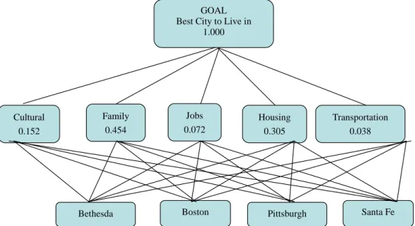
6. An Example of an AHP Decision
The simple decision is to choose the best city in which to live. We shall show how to make this decision using both methods of the AHP which conform with what Blumenthal said. We do it first with relative (comparative) measurement and second with absolute
measurement. With the relative measurement method the criteria are pairwise compared with respect to the goal, the alternatives are pairwise compared with respect to each criterion and the results are synthesized or combined using a weighting and adding process to give an overall ranking of the alternatives. With the absolute measurement method standards are established for each criterion and the cities are
rated one-by-one against the standards rather than being compared with each other.
6.1 Making the Decision with a Relative Measurement Model
The relative measurement model for picking the best city in which to live is shown below in Figure 4 (example by Mary Reiter).
Bethesda Boston Pittsburgh Santa Fe GOAL
Best City to Live in 1.000
Cultural 0.152
Family 0.454
Jobs 0.072
Housing 0.305
Transportation 0.038
Figure 4 Relative model for choosing best city to live in
Entering Judgments
For each cell in the comparison matrix there is associated a row criterion (listed on the left), call it X, and a column criterion (on the top), call it Y. One answers this question for the cell: How much more important is X than Y in choosing a best city in which to live? The judgments, shown in Table 3, are entered using the Fundamental Scale of the AHP. Fractional values between the integers such as 4.32 can also be used when they are known from measurement.
The Number of Judgments and Consistency In this decision there are 10 judgments to be entered. As we shall see later, inconsistency for a judgment matrix can be computed as a function of its maximum eigenvalueλmax and the order n of the matrix. The time gained, from making fewer judgments than 10 along a spanning tree for example can be offset by not having sufficient redundancy in the judgments to fine tune and improve the overall outcome.
There can be no inconsistency when the minimum number of judgments is used.
Next the alternatives are pairwise compared with respect to each of the criteria. The judgments and the derived priorities for the alternatives are shown in Table 4. The priority vectors are the principal eigenvectors of the pairwise comparison matrices. They are in the distributive form, that is, they have been normalized by dividing each element of the principal eigenvector by the sum of its elements so that they sum to 1. The priority vectors can be transformed to their idealized form by selecting the largest element in the vector and dividing all the elements by it so that it takes on the value 1, with the others proportionately less. The element (or elements) with a priority of 1 become the ideal(s). Later we explain why we use these two forms of synthesis.
Synthesis
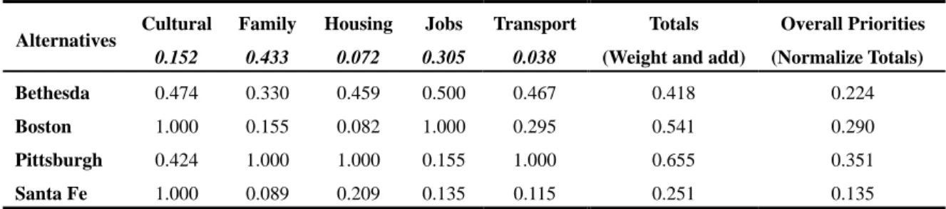
The outcome of the distributive form is shown in Table 5 and that for the ideal form is shown in Table 6. The columns in Table 5 are the priority vectors for the cities from Table 4
and the columns in Table 6 are these same vectors in idealized form with respect to each criterion. Using either form the totals vector is obtained by multiplying the priority of each criterion times the priority of each alternative with respect to it and summing. The overall priority vector is obtained from the totals vector by normalizing: dividing each element in the totals vector by the sum of its elements.
The final outcome with either form of synthesis is that Pittsburgh is the highest ranked city for this individual. Though the final priorities are somewhat different the order is the same: Pittsburgh, Boston, Bethesda and Santa Fe. The ratios of the final priorities are meaningful. Pittsburgh is almost twice as preferred as Bethesda.
When synthesizing in the distributive form the totals vector and the overall priorities vector are the same. When synthesizing in the ideal form as shown in Table 6 they are not.
Ideal synthesis gives slightly different results from distributive synthesis in this case.
Table 3 Criteria weights with respect to the goal
GOAL Culture Family Housing Jobs Transportation Priorities
Culture 1 1/5 3 1/2 5 0.152
Family 5 1 7 1 7 0.433
Housing 1/3 1/7 1 1/4 3 0.072
Job 2 1 4 1 7 0.305
Transportation 1/5 1/7 1/3 1/7 1 0.038 Inconsistency 0.05
Table 4 Alternatives’ weights with respect to criteria
Culture Bethesda Boston Pittsburgh Santa Fe Priorities
Bethesda 1 1/2 1 1/2 0.163
Boston 2 1 2.5 1 0.345
Pittsburgh 1 1/2.5 1 1/2.5 0.146
Santa Fe 2 1 2.5 1 0.345
Inconsistency .002
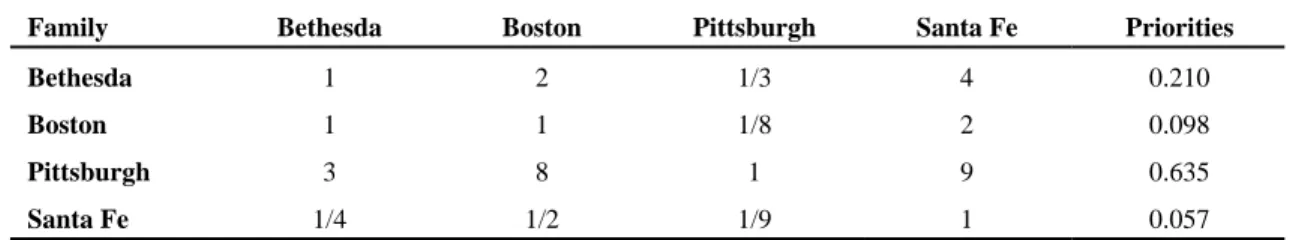
Family Bethesda Boston Pittsburgh Santa Fe Priorities
Bethesda 1 2 1/3 4 0.210
Boston 1 1 1/8 2 0.098
Pittsburgh 3 8 1 9 0.635
Santa Fe 1/4 1/2 1/9 1 0.057
Inconsistency .012
Housing Bethesda Boston Pittsburgh Santa Fe Priorities
Bethesda 1 5 1/2 2.5 0.262
Boston 1/5 1 1/9 1/4 0.047
Pittsburgh 2 9 1 7 0.571
Santa Fe 1/2.5 4 1/7 1 0.120
Inconsistency .012
Jobs Bethesda Boston Pittsburgh Santa Fe Priorities
Bethesda 1 1/2 3 4 0.279
Boston 2 1 6 8 0.559
Pittsburgh 1/3 1/6 1 1 0.087
Santa Fe 1/4 1/8 1 1 0.075
Inconsistency .004
Transportation Bethesda Boston Pittsburgh Santa Fe Priorities
Bethesda 1 1.5 1/2 4 0.249
Boston 1/1.5 1 1/3.5 2.5 0.157
Pittsburgh 2 3.5 1 9 0.533
Santa Fe 1/4 1/2.5 1/9 1 0.061
Inconsistency .001
Table 5 Synthesis using the distributive mode to obtain the overall priorities for the alternatives
Synthesis Cultural 0.152
Family 0.433
Housing 0.072
Jobs 0.305
Transport 0.038
Totals (Weight and add)
Overall Priorities (Normalize Totals) Bethesda 0.163 0.210 0.262 0.279 0.249 0.229 0.229 Boston 0.345 0.098 0.047 0.559 0.157 0.275 0.275 Pittsburgh 0.146 0.635 0.571 0.087 0.533 0.385 0.385 Santa Fe 0.345 0.057 0.120 0.075 0.061 0.111 0.111
Table 6 Synthesis using the ideal mode to obtain the overall priorities for the alternatives
Alternatives Cultural 0.152
Family 0.433
Housing 0.072
Jobs 0.305
Transport 0.038
Totals (Weight and add)
Overall Priorities (Normalize Totals) Bethesda 0.474 0.330 0.459 0.500 0.467 0.418 0.224 Boston 1.000 0.155 0.082 1.000 0.295 0.541 0.290 Pittsburgh 0.424 1.000 1.000 0.155 1.000 0.655 0.351 Santa Fe 1.000 0.089 0.209 0.135 0.115 0.251 0.135
Ideal Synthesis Prevents Rank Reversal (Saaty 2001, Saaty and Vargas 1984a)
An important distinction to make between measurement in physics and measurement in decision making is that in the first we usually seek measurements that approximate to the weight and length of things, whereas in human action we seek to order actions according to priorities. In mathematics a distinction is made between metric topology that deals with the measurement of length, mass and time and order topology that deals with the ordering of priorities through the concept of dominance rather than closeness used in metric methods.
We have seen that the principal eigenvector of a matrix is necessary to capture dominance priorities. When we have a matrix of judgments we derive its priorities in the form of its principal eigenvector. When we deal with a hierarchy the principle of hierarchic composition involves weighting and adding as a special case of the more general principle of network composition in which priorities are also derived as the principal eigenvector of a stochastic matrix which involves weighting and adding in the process of raising a matrix to powers. Some scholars whose specialization is in the physical sciences are perhaps unaware of the methods of order topology and have used various arguments to justify why they would
use a metric approach to derive priorities and also to obtain the overall synthesis. It may be worthwhile to discuss this at some length in the following paragraph.
Ideal synthesis should be used when one wishes to prevent reversals in rank of the original set of alternatives from occurring when a new dominated alternative is added.
With the distributive form rank reversal can occur to account for the presence of many other alternatives in cases where adding many things of the same kind or of nearly the same kind can depreciate the value of any of them. It has been established that 92% of the time, there is no rank reversal in the distributive mode when a new dominated alternative is added (Saaty and Vargas 1993). We note that uniqueness or manyness are not criteria that can be included when the alternatives are assumed to be independent of one another, for then to rank an alternative one would have to see how many other alternatives there are thus creating dependence among them.
Both the distributive and ideal modes are necessary for use in the AHP. We have shown that idealization is essential and is independent of what method one may use. There are people who have made it an obsession to find ways to avoid rank reversal in every decision and wish to alter the synthesis of the AHP away from
normalization or idealization. They are likely to obtain outcomes that are not compatible with what the real outcome of a decision should be, because in decision-making we also want uniqueness of the answer we get.
Here is a failed attempt by some people to do things their metric way to preserve rank other than by the ideal form. The multiplicative approach to the AHP uses the familiar methods of taking the geometric mean to obtain the priorities of the alternatives for each criterion without normalization, and then raising them to the powers of the criteria and again taking the geometric mean to perform synthesis in a distorted way to always preserve rank. It is essentially a consequence of attempting to minimize the logarithmic least squares expression (Saaty 2000a, Saaty and Vargas 1984b)
2
1 1
log log
n n i
i j ij j
a w
w
= =
−
∑ ∑
.
It does not work when the same measurement is used for the alternatives with respect to several criteria as one can easily verify and that should be sufficient to throw it out. Second and more seriously, the multiplicative method has an untenable mathematical problem. Assume that an alternative has a priority 0.2 with respect to each of two criteria whose respective priorities are 0.3 and 0.5. It is logical to assume that this alternative should have a higher priority with respect to the more important criterion, the one with the value of 0.5, after the weighting is performed. But 0.20.5<0.20.3 and alas it does not, it has a smaller priority. One would think that the procedure of ranking in this way would have been abandoned at first knowledge
of this observation.
We conclude that in order to preserve rank indiscriminately from any other alternative, one can use the rating approach of the AHP described below in which alternatives are evaluated one at a time using the ideal mode.
In addition, by deriving priorities from paired comparisons, rank is always preserved if one idealizes only the first time, and then compares each alternative with the ideal, allowing the value to exceed one. On the other hand, idealizing repeatedly, only preserves rank from irrelevant alternatives.
Remark On occasion someone has suggested the use of Pareto optimality instead of weighting the priorities of the alternatives by the priorities of the criteria and adding to find the best alternative. It is known that a concave function for the synthesis, if one could be found, would serve the purpose of finding the best alternative when it is known what it should be. But if the best alternative is already known for some property that it has which makes it the best, then one has a single not a multiple criteria decision. Naturally a multiple criteria problem may not yield the expected outcome. This is a special case of when the weights of the criteria depend on those of the alternatives. We will see in Part 2 that the final overall choice is automatically made in the process of finding the priorities of the criteria as they depend on the alternatives. Pareto optimality plays no role to determine the best outcome in that general case.
6.2 Making the Decision with an Absolute or Ratings Model
Using the absolute or ratings method of the AHP, categories (intensities) or standards are established for the criteria and cities are rated one at a time by selecting the appropriate
category under each criterion rather than compared against other cities. The standards are prioritized for each criterion by making pairwise comparisons. For example, the standards for the criterion Job Opportunities are: Excellent, Above Average, Average, Below Average and Poor. Judgments are entered for such questions as: “How much more preferable is Excellent than Above Average for this criterion? Each city is then rated by selecting the appropriate category for it for each criterion. The city’s score is then computed by weighting the priority of the selected category by the priority of the criterion and summing for all the criteria. The prioritized categories are essentially absolute scales, abstract yardsticks, which have been derived and are unique to each criterion.
Judgment is still required to select the
appropriate category under a criterion for a city, but the cities are no longer compared against each other. In absolute measurement, the cities are scored independently of each other. In relative measurement, there is dependence, as a city’s performance depends on what other cities there are in the comparison group. Figure 5 and Tables 7, 8 and 9 represent what one does in the ratings or absolute measurement approach of the AHP. Table 7 illustrates the pairwise comparisons of the intensities under one criterion. The process must be repeated to compare the intensities for each of the other criteria. We caution that such intensities and their priorities are only appropriate for our given problem and should not be used with the same priorities for all criteria nor carelessly in other problems.
GOAL
Best City to Live in 1.000
Cultural 0.152
Family 0.454
Housing 0.072
Jobs 0.305
Transportation 0.038 Extreme
1.000 Great .411 Significant .188 Moderate .106
Tad .052
Abundant .906 Considerable 1.000 Manageable .396 Negligible .120 Own<35% Sal.
1.000 Own>35% Sal.
.363 Rent<35% Sal.
.170
Rent>35% Sal.
.056
Excellent 1.000
Average .306
Poor .065
<100 mi 1.000 101-300 mi .521 301-750 mi .179
>750 mi .079
Above Avg .664
Below Avg .126
Figure 5 Absolute or ratings mode for choosing best city to live in
Table 7 Deriving priorities for the cultural criterion categories Extreme Great Significant Moderate Tad Derived
Priorities
Idealized Priorities
Extreme 1 5 6 8 9 .569 1.000
Great 1/5 1 4 5 7 .234 .411
Significant 1/6 1/4 1 3 5 .107 .188
Moderate 1/8 1/5 1/3 1 4 .060 .106
Tad 1/9 1/7 1/5 1/4 1 .030 .052
Inconsistency = .112
Table 8 Verbal ratings of cities under each criterion Alternatives Cultural
.195
Family .394
Housing .056
Jobs .325
Transport .030
Total Score
Priorities (Normal.) Pittsburgh Signific. <100 mi Own>35% Average Manageable .562 .294 Boston Extreme 301-750 mi Rent>35% Above Avg Abundant .512 .267 Bethesda Great 101-300 mi Rent<35% Excellent Considerable .650 .339 Santa Fe Signific. >750 mi Own>35% Average Negligible .191 .100
Table 9 Priorities of ratings of cities under each criterion Alternatives Cultural
.195
Family .394
Housing .056
Jobs .325
Transport .030
Total Score
Priorities (Normalized) Pittsburgh 0.188 1.000 0.363 0.306 0.396 .562 .294 Boston 1.000 0.179 0.056 0.664 0.906 .512 .267 Bethesda 0.411 0.521 0.170 1.000 1.000 .650 .339 Santa Fe 0.188 0.079 0.363 0.306 0.120 .191 .100
When the intensities are intangible, like excellent, very good and so on down to poor, there may be alternatives that fall above or below that range because what is excellent for one group of alternatives may not be applicable to alternatives that are much better or much worse than the given alternatives. In that case we need to expand the intensities by putting them into categories. We may use the same names for them but we may have order of magnitude categories in which we compare the elements in each category or even use the same scale but then combine that category with
an adjacent category using the top or bottom rated intensity as a pivot as in the cherry and watermelon example. To determine which category an alternative should be rated on, we first start with any alternative and rate it. From then on before rating a new alternative we need to compare it with the previous alternative if it is better or worse and in doing that we need to reason through and insert hypothetical alternatives to place it correctly just as we did in the cherry-watermelon example. In real life, alternatives that naturally occur in a certain activity tend to be alike or homogeneous. Even
when they are not alike they generally differ by one or two categories of intensity on each criterion. When they differ by more, they are unlikely to be considered as serious contenders and are assigned a zero value. The concern is usually from the top rated alternatives downwards for the intensities of each criterion.
7. Sanctioning China? An Application with Benefits, Costs and Risks
This example was developed in February 1995 when media were voicing strong opinion about whether the US government should sanction China about intellectual property rights. I and my coauthor Professor Jen Shang
sent our analysis to Mr. Mickey Kantor, the then chief US negotiator before his trip to Beijing. Mr. Kantor acknowledged reading our article in a very positive way by calling me.
We are not taking credit that the US did not sanction China. But we are quite happy that the outcome of the decision was along the lines of our recommendation. The model we used, shown in Figure 6, is a three part Benefits, Costs and Risks model. Note that in this example we formed the (marginal) ratio of the benefits which are positive, to the costs and risks both of which are opposite because we must respond to the question, which alternative is more costly (risky) for a give criterion.
Protect rights and maintain high Incentive to make and sell products in China (0.696)
Rule of Law Bring China to responsible free-trading 0.206)
Help trade deficit with China (0.098)
BENEFITS
Yes 0.729 No 0.271
$ Billion Tariffs make Chinese products more expensive (0.094)
Retaliation (0.280)
Being locked out of big infrastructure buying: power stations, airports (0.626) COSTS
Yes 0.787 No 0.213
Long Term negative competition (0.683)
Effect on human rights and other issues (0.200)
Harder to justify China joining WTO (0.117)
RISKS
Yes 0.597 No 0.403
Result: Benefits
Costs x Risks; YES .729
.787 x .597 = 1.55 NO .271
.213 x .403 = 3.16 Yes
No .80 .20
Yes No
.60 .40
Yes No
.50 .50
Yes No
.70 .30
Yes No
.90 .10
Yes No
.75 .25
Yes No
.70 .30
Yes No
.30 .70
Yes No
.50 .50
Figure 6 China trade sanction model
8 7 6 5 4 3 2 1
Benefits/Costs*Risks
Experiments
0 30 60 90 120 150 1 80 210
No Yes
..
. . .
. ..
. . ....
.. . . .
. .
. ... ..
. ...
. .
... .
Figure 7 Sensitivity analysis of the outcome of the China decision In later examples, instead of forming ratios
of absolute numbers, we use subtraction and negative priorities (Saaty and Ozdemir 2003b) after carefully rating one at a time the highest ranked alternative under each of the benefits (B), opportunities (O), the costs (C) and the risks (R) or as a collective we refer to them as (BOCR). The highest ranked alternative is often different under each. In this manner instead of obtaining marginal (per unit) results by forming the ratio we obtain the totals. It is clear from this analysis that the US should not have taken any action that would be averse to cultivating a successful working relation between the two great countries for the foreseeable future.
8. Stimulus-Response and the Fundamental Scale
We shall see in Part 2 that a hierarchy is a special case of a network whose priorities and interactions are represented in a supermatrix W.
As a result, hierarchic synthesis of priorities is a special case of network synthesis of priorities (Saaty 2001). The limit priorities of W, limit as
of k,
k→ ∞ W yield its network synthesis.
Equivalently, because W is column stochastic, its network synthesis can be obtained by solving the principal eigenvalue problem
with max 1.
Ww w= λ = Invariance of the eigenvector makes additive hierarchic synthesis necessary to obtain priorities for a hierarchy.
To be able to perceive and sense objects in the environment our brains miniaturize them within our system of neurons so that we have a proportional relationship between what we perceive and what is out there. Without proportionality we cannot coordinate our thinking with our actions with the accuracy needed to control the environment.
Proportionality with respect to a single stimulus requires that our response to a proportionately amplified or attenuated stimulus we receive from a source should be proportional to what our response would be to the original value of that stimulus. If w(s) is our response to a stimulus of magnitude s, then the foregoing gives rise to the functional equation w(as) = b w(s). This equation can also
be obtained as the necessary condition for solving the Fredholm equation of the second kind:
( ) ( ) max ( )
b
aK s,t w t dt = λ w s
∫
obtained as the continuous generalization of the discrete formulation Aw=λmaxw for deriving priorities where instead of the positive reciprocal matrix A in the principal eigenvalue problem, we have a positive kernel, K(s,t) > 0, with K(s,t) K(t,s) = 1 that is also consistent i.e.
K(s,t) K(t,u)= K(s,u), for all s, t, and u . The solution of this functional equation in the real domain is given by
log log
log log
( ) log
b s
a s
w s Ce P
a
=
where P is a periodic function of period 1 and P(0) = 1. One of the simplest such examples with u=log / logs ais P(u) = cos (u/2Β) for which P(0) = 1.
The logarithmic law of response to stimuli can be obtained as a first order approximation to this solution through series expansions of the exponential and of the cosine functions as:
1 2 3
( ) u ( ) log
v u =C e−β P u ≈C s C+
logab≡ −β β, >0. The expression on the right is known as the Weber-Fechner law of logarithmic response M =alogs b a+ , ≠0 to a stimulus of magnitude s. This law was empirically established and tested in 1860 by Gustav Theodor Fechner who used a law formulated by Ernest Heinrich Weber regarding discrimination between two nearby values of a stimulus. We have now shown that that Fechner’s version can be derived by
starting wit