No part of this book may be reproduced, stored in a retrieval system, or transmitted in any form or by any means: electronic, electrostatic, magnetic, tape, mechanical photocopying, recording, or otherwise without the written permission of the Publisher. The performance of the control schemes, implemented on the Leonard underwater vehicle for 3D helical trajectory tracking, is then demonstrated through scenario-based numerical simulations.
A DAPTİVE A DJUSTMENT OF P ROCESS N OİSE
C OVARİANCE İN K ALMAN F İLTER FOR E STİMATİON OF AUV D YNAMİCS
I NTRODUCTION
One of the methods for constructing such an algorithm is to use a single adaptive factor as a multiplier for the process or measurement noise covariance matrices [5, 9]. In this case, by using a measurement noise scale factor (MNSF) as a multiplier on the measurement noise covariance matrix, the insensitivity of the filter to the current measurement errors can be satisfied.
M ATHEMATICAL M ODEL OF A UTONOMOUS
- Diving Subsystem of Sample AUV Model
- Discretization for Diving Subsystem Diving subsystem matrices are given below;
- Steering Subsystem of Sample AUV
- Discretization of Steering Subsystem
Discretization for the diving subsystem The diving subsystem matrices are given below; The dive subsystem matrices are given below; The mathematical model of the diving subsystem can be rewritten in matrix form as;.
K ALMAN F ILTER FOR E STIMATION OF AUV D YNAMICS
- Optimum Linear Kalman Filter Equations
- Adaptive Fading Kalman Filter
- Adaptive Fading KF with Single Fading Factor
- Adaptive Fading KF with Multiple Fading Factor
The presented adaptive KF will ensure guaranteed adaptation of the filter to changing system operating conditions. In this case, the real and theoretical values of the innovation covariance matrix should be compared again.
S IMULATION R ESULTS
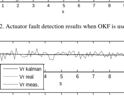
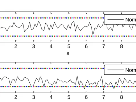
- OKF Results
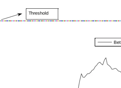
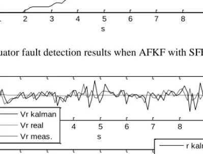
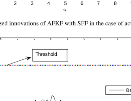
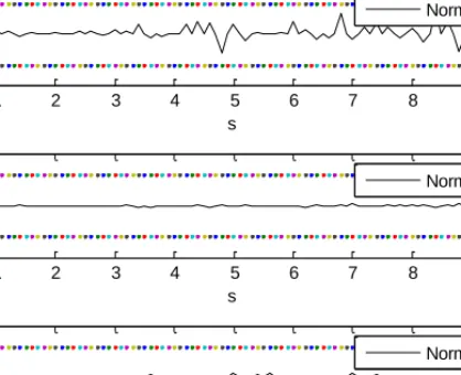
- AFKF with SFF Simulation Results
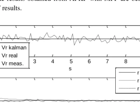
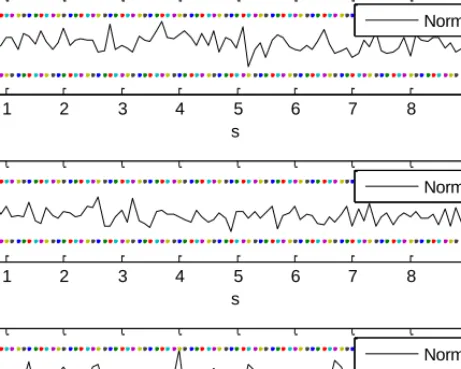
- AFKF with MFF Simulation Results
The control distribution matrix of the system has been changed to simulate the event of an actuator failure. This study is mainly focused on the application of the adaptive Kalman filter algorithm to the dynamics estimation of high-speed autonomous underwater vehicles.
F ROM N ON -M ODEL -B ASED TO A DAPTIVE
M ODEL -B ASED T RACKING C ONTROL OF
L OW -I NERTIA U NDERWATER V EHICLES
I NTRODUCTION Context
Motivated by underwater challenges as well as the high demand for raw materials, research communities proposed using divers to explore and exploit this environment. These missions may require the vehicle's ability to autonomously make an intelligent decision. Focusing on trajectory tracking and station-keeping problems, some of the proposed classical non-model-based controllers include: classical PD and PID control schemes for position and velocity regulation of a fully actuated AUVs, respectively, which have been proposed in [9].
To improve the performance of the classical PID controller for tracking control of mini-ROVs in subsea applications, the idea of auto-adjustment of the feedback gains using neural networks was proposed in [17]. Although the authors demonstrated the performance of the control scheme through simulations and real-time experiments, the neural networks are always associated with long training time and high computational cost. The performances of the proposed control schemes are evaluated through real-time experiments using Johns Hopkins University remotely operated vehicle (JHU-ROV).
However, the computation time of the proposed controllers can be reduced by using the desired compensation in the control schemes, which can be calculated offline. The results obtained show the better performance of the non-linear model-based controller compared to a non-model-based controller.
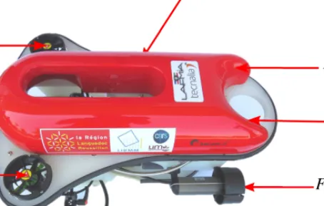
V EHICLE D ESCRIPTION AND M ODELLING 1. Vehicle Description
In this chapter, we propose to investigate the design, stability analysis, and performance of tracking control schemes, from model-free to model-based and adaptive models, and their application to the control of a low-inertia underwater vessel. a vehicle for naval missions. These vehicles are characterized by a high power-to-weight ratio, which makes them vulnerable to any minor change in system parameters. Section 2 presents the description of the low-inertia underwater vehicle and its six-degree-of-freedom modeling.
Allocation view of the Leonard underwater vehicle's thrusters, which produce the forces responsible for the vehicle's navigation. The kinematics and dynamics of a low-inertia underwater vehicle such as Leonard can be derived relative to 3D reference frames. The total contributions of the inertia of the rigid body MRB of the vehicle and the inertia of the added mass MA constitute the so-called inertia matrix M.
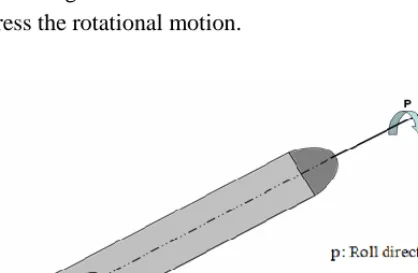
The detailed step-by-step process to obtain approximate values of the hydrodynamic elements (Xu, Yv, Zw, Kp, Mq, Nr) of the vehicle's D(ν) matrix is addressed in [34]. We finalize the description of the vehicle's dynamics terms withτ, which is a control input vector responsible for the translational and rotational motions of the vehicle.
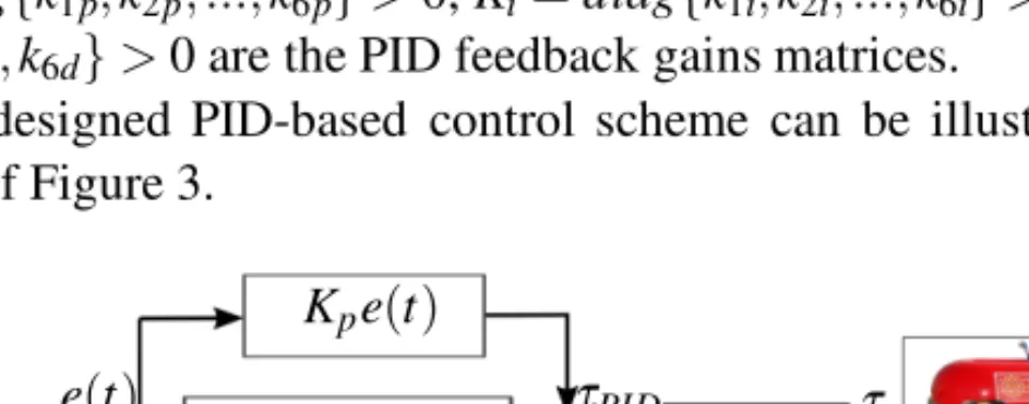
P ROPOSED C ONTROL S OLUTIONS AND T HEIR S TABILITY A NALYSIS
On the other hand, non-optimal gain selection can lead to the instability of the resulting closed loop dynamics. Block diagram of the non-model based PID control scheme implemented on the Leonard submersible vehicle. In accordance with LaSalle's principle of invariance, the origin of the resulting closed-loop dynamics is asymptotically stable [34], [40].
However, the CT control scheme has the advantage of transforming the closed-loop dynamics of the nonlinear system into a linear closed-loop dynamics. The block diagram of the CT controller structure implemented in the Leonard underwater vehicle is illustrated in Figure 4. We exploit this property of the vehicle dynamics and focus on designing Φϑandϑ based on the terms (i.e. wext(t) and g?(η) ) which significantly affect the steady state of the vehicle as follows [35].
The structure of the proposed APD+ control scheme implemented on the Leonard submersible is illustrated in Figure 5. Therefore, we can conclude that the origin of the resulting closed-loop dynamics is asymptotically stable.
S IMULATION R ESULTS : A C OMPARATIVE S TUDY To compare the effectiveness and robustness of the proposed three controllers
Comparison of tracking performance of APD+, CT and PID controllers implemented on the Leonard underwater vehicle in a nominal scenario:. top diagrams) yaw and pitch tracking, (middle diagrams) the corresponding yaw and pitch tracking errors, and (bottom diagrams) are the development of inputs for vehicle yaw and pitch control. Comparison of tracking performance of APD+, CT and PID controllers implemented on the Leonard underwater vehicle in a nominal scenario:. top plots) pitch and yaw tracking, (middle plots) the corresponding pitch and yaw tracking errors, and (bottom plots) are the evolution of vehicle pitch and yaw control inputs. Comparison of the three-dimensional (3D) helical trajectory tracking performance of the APD+, CT and PID controllers implemented on the Leonard underwater vehicle in a nominal scenario.
Parametric evaluations of the APD+ controller implemented on the Leonard underwater vehicle for three-dimensional (3D) helical trajectory tracking in a nominal scenario. Comparison of tracking performance of APD+, CT and PID controllers implemented on the Leonard underwater vehicle in a combined scenario:. top diagrams) yaw and pitch tracking, (middle diagrams) the corresponding yaw and pitch tracking errors, and (bottom diagrams) are the development of inputs for vehicle yaw and pitch control. Comparison of three-dimensional (3D) helical trajectory tracking performance of APD+, CT, and PID controllers implemented on the Leonard underwater vehicle in a combined scenario.
Parametric estimates of the APD+ controller implemented on Leonard underwater vehicle for three-dimensional (3D) helical trajectory tracking in the combined scenario. External perturbation estimation of the APD+ controller implemented on Leonard underwater vehicle for three-dimensional (3D) helical trajectory tracking in the combined scenario.
C ONTROLLERS TO A VOID C OLLISION WITH 3D O BSTACLES U SING S ENSORS
P RELIMINARY I NFORMATION 1. Model
In this chapter, two reference systems are used: the inertial reference system {I} and the body-mounted reference system {B} [24]. The counterclockwise rotation of ψ around the z-axis in the inertial coordinate system is represented by the following rotation matrix R(ψ). A counterclockwise rotation of θ around an axis in an inertial coordinate system is represented by the following rotation matrix R(θ).
The counterclockwise rotation of φ about the x-axis in the inertial coordinate system is represented by the following rotation matrix (φ).
D EFINITIONS AND A SSUMPTIONS
We say that the vehicle collides with an obstacle point if the relative distance between the vehicle and the obstacle point is less than r. To avoid a collision with an obstacle, it is assumed that the detection range of a vehicle is greater thanr. 1The speed of an obstacle point is that of an obstacle whose obstacle point is on its limit.
We can track an obstacle point with functions to estimate the speed of the corresponding obstacle. However, estimating the speed of an obstacle is beyond the scope of this chapter. Since we consider a 3D sensor with a large measurement error, we must set a large value.
C ONTROL L AWS FOR C OLLISION A VOIDANCE 1. Collision Prediction
In the case where dmin is greater than r, the vehicle avoids the collision within U steps, using the basic collision avoidance condition. In the case where the collision avoidance condition is not met for at least one obstacle point, the vehicle requires a safe speed to avoid the collision. Once a collision avoidance maneuver is initiated in the time step, the vehicle does not move to the goal directly by timesteps+I.
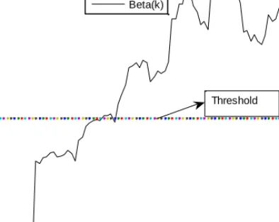
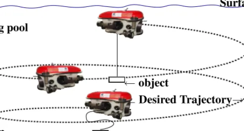
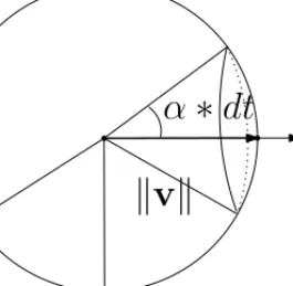
The idea of these maneuvers is to search for a speed that meets the collision avoidance condition, followed by using the speed to move the vehicle in one time step. Here h(k, j) denotes the jth element of h(k). 15) We use numerical methods to search for a safe speed vector in time step k+1 to avoid collisions. The velocity vector of the vehicle in the body-mounted frame is (v(k),0,0), which is shown in Figure 1 as a bold arrow.
This implies that we cannot find a safe velocity vector that guarantees collision avoidance within time steps in the future. In case the above condition is met, we use to control the vehicle within one time step.
MATLAB S IMULATIONS
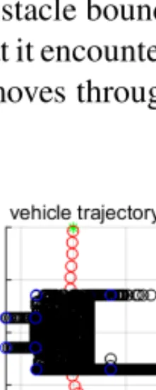
Watch the vehicle change its attitude and speed to avoid collision as it approaches the goal. The yaw, pitch and speed of the vehicle with respect to time, considering the scenario in Figure 2. Note that the vehicle changes its attitude and speed to avoid colliding with obstacles while approaching the goal.
Violation, pitch and speed of the vehicle with respect to time, considering the scenario in Figure 5. Since we set dt= 5 seconds, the trajectory of the vehicle is smoothed less than the case kudt = 1 second. Violation, pitch and speed of the vehicle with respect to time, considering the scenario in Figure 8.
The yaw rate, angle and speed of the vehicle in relation to time, taking into account the scenario in Figure 11. Our control laws are designed taking into account the maximum turn rate and the maximum speed of the vehicle.
I NDEX