99 6.5 (a-c) The two terminal spin polarized conductance, Gsz is plotted as a. function of the Fermi energy in the absence of Rashba SOC for three different adatom concentrations, namely nad and 0.1. d-f) Their corresponding fluctuations are plotted as a function of E. 6.8 (a) The local charge current,J0 and (b) diez component of the local spin current are shown in the absence of Rashba SOC. 105 6.12 (a-c) The four terminal spin polarized conductance, Gsz is plotted as . a function of the Fermi energy, E in the absence of Rashba SOC for three different adatom concentrations.
The behavior of the total DOS is plotted as a function of the Fermi energy (c) for λR = 0 and (e) for λR=0.2.
Spin-orbit interaction
Dresselhaus spin-orbit interaction
Dresselhaus observed that in III-V zinc-blende semiconductor compounds that do not have an inversion center, such as GaAs, InSb, etc., the SO coupling near the Γ point has the form,. Considering the additional symmetry in the band structure results in additional coupling terms of odd SO [74].
Rashba spin-orbit interaction
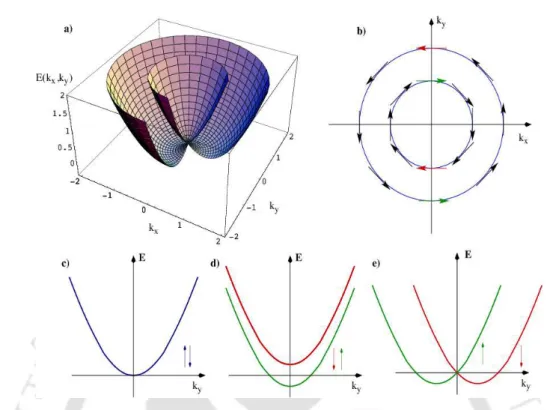
In Fig.1.1(c-e) energy spectra are presented as a function of this for different physical situations as explained below. In the presence of a magnetic field B~ (Fig.1.1(d)), spin degeneracy is raised by Zeeman splitting and the gap separating up and down spin is equal to gµBB where g is the Bohr magneton.
Discretization scheme for the Hamiltonian
Junction devices
Basics of Graphene
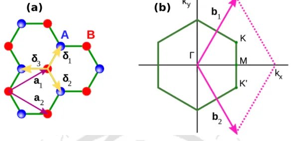
Crystal structure
The vectors δ1, δ2 and δ3 connect the carbon atoms to each other at a distance of a = 1.42 ˚A. Vectors a1 and a2 are base vectors. The positions of the two (non-equivalent) Dirac points K and K′ located at the corners of the Brillouin zone (as shown in Figure 1.3(b)) are,.
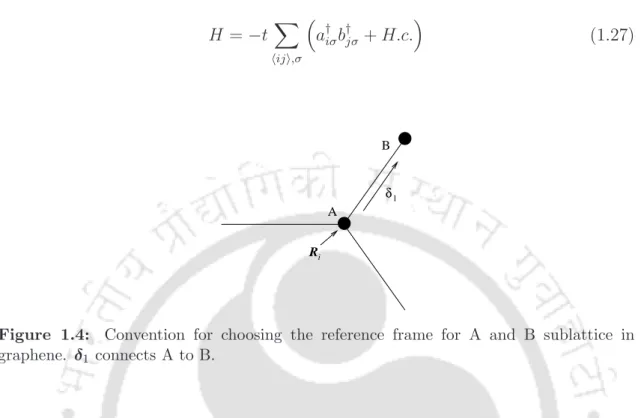
Tight-binding approximation
It is convenient to write the tight-binding eigenfunctions in the form of a spinor whose components correspond to the amplitudes of the A and B atoms respectively in the unit cell, marked with a reference point R0i. It is a matter of convention how we choose the pair A and B and the point R0i, but for the sake of accuracy let us choose that B should be separated from A by δ1 and R0i at the position of A as shown in Fig.1.4.
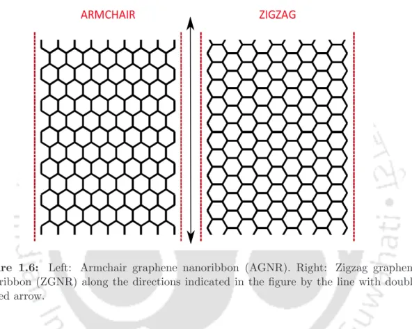
Graphene Nanoribbon
It should also be noted that the width of the AGNR has a zigzag shape and a ZGNR also has the shape of an armchair. The electronic properties of GNRs depend on the geometry of the edges and the lateral width of the nanoribbons.
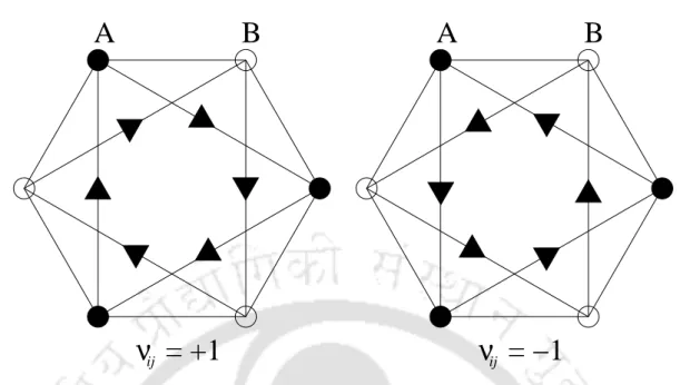
Kane-Mele model
The third term is the mirror-symmetric spin-orbit interaction involving spin-dependent second neighbor hopping. The fourth term is the closest Rashba term, which violates z → −z mirror symmetry and is a known component for our discussion.
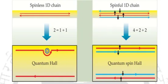
Quantum spin Hall effect
The QSH state can be viewed as two copies of the QH state, one for each spin with opposite Hall conduction. In contrast, the QSH state can be qualitatively thought of as two copies of the QH state, with one copy for each spin. Spatial separation is achieved in the case of the QSH effect via the invariant spin-orbit coupling TR.
However, both ideas provide the important conceptual framework within which the stability of the QSH state can be investigated. The condition for the wave functions to be exact at E = 0 is that the total sum of the components. The inclusion of the magnetic adatoms can be included by an external exchange bias in the Kane–Mele Hamiltonian (where the intrinsic SOC is absent for magnetic adatoms).
The local load current and the local torque current provide an intuitive idea of the conduction properties of the system. RSOC is found to have a detrimental effect on the width of Hall plateaus. From the Fisher-Lee relation[100], the elements of the distribution matrix S can be obtained from the Green's function.
Transmission function and Scattering matrix
To ensure current conservation, the S-matrix must be uniform and therefore must satisfy the condition.
Transmission coefficients and the Green’s Function
Green’s Function formalism
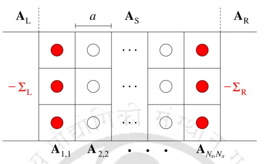
The system is divided into three regions: the scattering region, denoted by the matrix, AS, and two semi-infinite leads, AL and AR. The effects of the semi-infinite leads are added as self-energies ΣL and ΣR to the points on the left and right boundaries of the scattering region. To do this, we divide the Hamiltonian for the entire system into three parts: the left and right leads, represented by the infinite-dimensional matrices AL and AR, respectively, and the scattering region denoted by AS, which is of finite size (Nx ×Ny), where Nx and Ny the number of discretized spatial points in the x and y directions of the scattering area (see Figure 2.2).
At the end of the calculations we will allow NL→ ∞ and NR → ∞ to obtain a continuous spectrum of eigenvalues for AL and AR[2].
Evaluation of the self-energy
M is the total number of transverse channels in the leads, and in our case M = Ny. The self-energy matrices are constructed in the reduced Hilbert space of the conductor itself. These matrices have non-zero elements only for the locations on the edge layer of the sample that are coupled to the leads and are given when the energy is out of band.
The recursive Green’s Function algorithm for two-terminal systems . 36
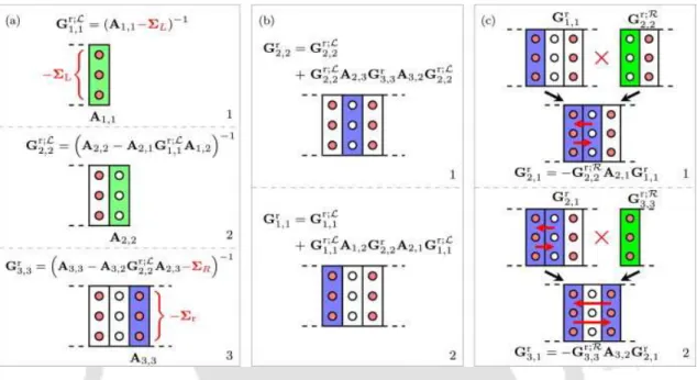
The first disk, which already contains the self-energy of the left wire, is flipped over and added to the next disk on the right. Since the last disc contains the self-energy of the right wire, the Green's function of the last disc is exact, that is GrNx,Nx = Gr;LNx,Nx. The algorithm can also be applied from right to left, which would produce right-connected Green's function marked with R. These right-connected Green's function will play a role in the last part of the algorithm. ii) The second part is called the backward algorithm and computes the diagonal blocks of the full Green's function.
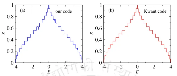
From the forward algorithm, we obtained the last block on the diagonal of the full Green's function. Using a discrete version of the Dyson equation, we can couple it to the left-connected Green's function Gr;LNx−1,Nx−1 of the adjacent disk on the left. In the absence of disorder, the conductance increases in discrete steps as we increase the Fermi energy for E < 0 and for E > 0 it decreases again in discrete steps, showing the quantum nature of the system.
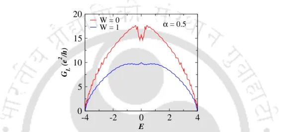
As the disorder is introduced, the step-like feature is lost and also the overall magnitude of the conductance decreases with increasing strength of disorder due to the scattering effects. The behavior of the normalized conductance is symmetric as a function of the Fermi energy, regardless of the perturbation strength. In the following, we have shown the behavior of normalized conductance as a function of the Fermi energy for a 16×16 square two-terminal scattering device.
Non-equilibrium Green’s function
System and the Hamiltonian
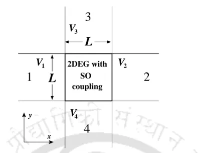
Here the four ideal (disorder-free) semi-infinite wires are attached to the central conducting region which in our case is a square lattice with Rashba spin-orbit interaction. The Hamiltonian for the entire system can be represented by a sum of three terms, namely: The first term represents the Hamiltonian for the system with a square lattice geometry with Rashba spin-orbit interaction and is defined by.
3.6) Here ǫi is the random potential energy at a site chosen from a uniform rectangular distribution (–W to W), c†i and ci correspond to the creation and annihilation operators, respectively, for the electron at site i of the conductor. m∗: effective mass and a0: lattice constant) is the jump integral, α is the Rashba coupling strength. Four metal wires attached to a conductor are considered semi-infinite and ideal. Thus, the leads are described by a similar non-interacting one-particle Hamiltonian as written below.
In the above expression, ǫLandtLdenotes site energies and nearest-neighbor hopping between the sites at the leads. The coupling between the conductor and the leads is defined by the hop integral tC. In Eq.(3.10) and m belong to the boundary locations of the square grid and conduits, respectively.
Formulation of longitudinal and spin Hall conductances
The transmission coefficient that appears above can be calculated in terms of the Green's function with the relation Γσp are the coupling matrices representing the coupling between the core region and the leads, and are defined by the relation [2]. 3.20). The self-energy contribution is calculated by modeling each terminal as a semi-infinite perfect wire [102]. It can be seen that the bias energy E controls the density of charge carriers flowing through the conduction region.
Throughout the thesis, when we refer to the conductance graphs (G) as a function of energy, we therefore imply Fermi energy. Now, according to the spin Hall phenomenology, the net charging currents through lead-3 and lead-4 are zero, that is, I3q = I4q = 0, because the transverse leads are voltage probes in our setup. On the other hand, since the currents in different lines depend only on the voltage differences between them, we can set any of the voltages to zero without any loss of generality. that the wires are connected with a geometrically symmetrical ordered bridge, so VV31 =. 3.24).
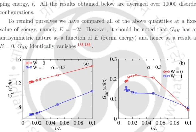
Results and discussion
The behavior of the spin Hall conductance of GSH is plotted as a function of the Fermi energy, as shown in Figure 3.8. Figure 5.10 shows the fluctuations in the spin polarized conductance, ∆Gsα, as a function of the Fermi energy. The variation of the spin Hall conductivity (in units of e/4π) as a function of the Fermi energy is shown in Figure 5.16(a).
However, the fluctuations in charge conductivity, ∆G are plotted as a function of Fermi energy separately, as shown in Fig.6.4 for clarity. Gsz, denoted by ∆Gsz, is plotted as a function of the Fermi energy, E as shown in Fig.6.5(d-f). The behavior of the corresponding fluctuations in the spin polarized conductance is shown in Fig.6.6(d-f).
Figure 6.8(a) shows the nature of the local charging current, J0 in the absence of Rashba SOC for a fixed value (near zero) of the Fermi energy, namely E =−0.09 (in units of t). The fluctuations of the spin Hall conductance are shown in Fig. 6.13(d-f) as a function of the Fermi energy. On the other hand, as shown in Figure 7.4(b), the maximum longitudinal conductivity increases in the presence of Rashba SOC.
Fig.7.7 shows the variation of the GSH spin Hall conductivity (in units of e/4π) as a function of the Fermi energy. Further, in the presence of a magnetic field, the behavior of the spin Hall conduction is studied.