Extratropics-to-tropics teleconnection and

I NTRODUCTION

M OTIVATIONS

Today, it is undeniable that climate change is one of the most critical challenges facing the planet. This introductory chapter starts by reviewing the theoretical foundations of the tropical general circulation (section 1.2) and various evidences for tropical-tropical teleconnection (section 1.3), organizes the development of an energetic framework (section 1.4), and finally presents a roadmap for the following chapters of the thesis (section 1.5).

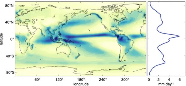
I NTER -T ROPICAL C ONVERGENCE Z ONE AND H ADLEY C IRCULATION

Therefore, it is natural that the dynamics and location of the ITCZ ​​were generally thought to be solely controlled by local climate features (Xie 2004). This dominant tropical rainfall pattern is part of the Hadley cell, a large-scale tropical atmospheric circulation.

E VIDENCE OF E XTRATROPICS - TO - TROPICS T ELECONNECTION

Lynch-Stieglitz 2004) and the western tropical Atlantic (Lea et al. 2003) show that the ITCZ ​​over both the Pacific and Atlantic basins shifted southward during the Last Glacial Maximum. Under the experiments of increasing and decreasing carbon dioxide, there is an irreversible shift of the ITCZ ​​in the Southern Hemisphere resulting from the delayed energy exchange in the Southern Ocean (Kug et al., 2021).

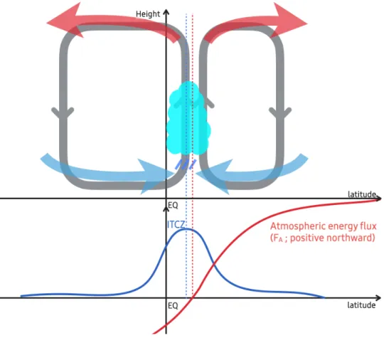
E NERGETIC FRAMEWORK

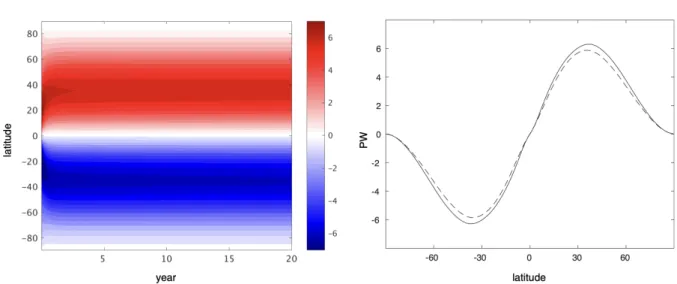
This framework suggests that the magnitude of the meridional shift of the ITCZ ​​is proportional to the transequatorial atmospheric energy transport (Broccoli et al. 2006; Kang et al. 2008), with the proportionality determined by the net input of energy to the tropical atmospheric column (Bischoff and Schneider 2014 ).

C HALLENGES AND R OADMAP

Although the magnitude of SST fluctuations is broadly similar in the extratropics (Figs. 2.2b and 2.3), the tropical rainfall response exhibits a strong sensitivity to the forcing period T (green-brown contours in Fig. 2.3). In all standard experiments (Fig. 2.5), the TOA radiation response a:R (black) is too small to make a noticeable impact on a:# as a result of cancellation between cloud a:0TU (black with points) and purity. -sky a: 0TR (black dot) component.

S ENSITIVITY OF THE T ROPICAL P RECIPITATION R ESPONSE TO

I NTRODUCTION

Specifically, the extratropics–tropics teleconnection has generally been taken into account when considering the steady state. In addition, section 2.4 presents the sensitivity of the extratropics–tropics teleconnection to the depth of the mixed layer.

Table 2.1. The standard deviation of inter-hemispheric difference in tropical (30°S~30°N) and extratropical (poleward of 30°S and 30°N) NEI in the GFDL-CM3 preindustrial experiment

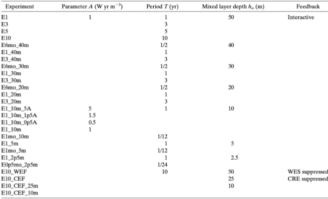
M ETHODOLOGY

In particular, experiment E10 is repeated with cloud properties (cloud water mixing ratio, cloud ice mixing ratio, and cloud fractional area) prescribed for a one-year time series arbitrarily chosen from the reference experiment at each 3 h in the radiative scheme (e.g., Kim et al. 2018). The amplitude parameter A determines the total amount of anomalous energy imposed on the plate ocean during half the period of the forcing T .

Figure 2.1. Zonal-mean Qflux (shading; W m -2 ) for E1

T HE ITCZ RESPONSE AND T RANSIENT E NERGETIC F RAMEWORK

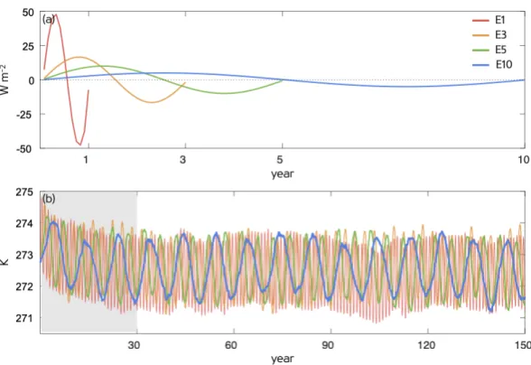
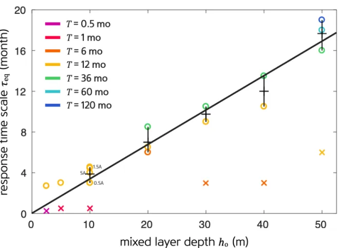
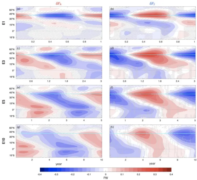
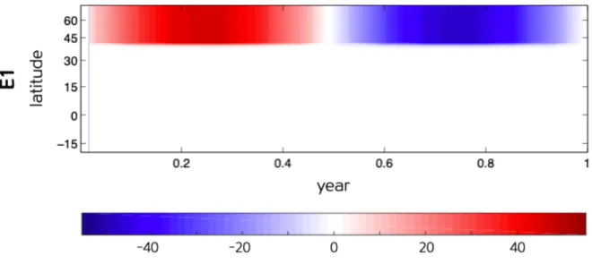
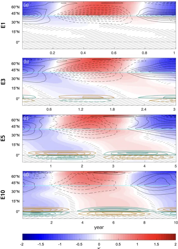
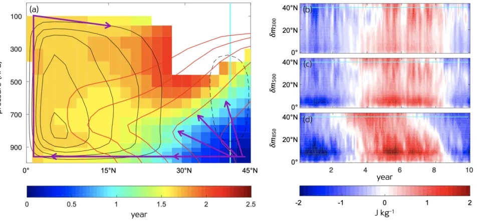
For the experiments without extratropical-to-tropical teleconnections, half of the forcing period T is indicated by cross symbols. For the experiments with the forcing amplitude different from A, the forcing amplitude is indicated by the text next to the symbols. In all experiments, a:S exhibits a clear oscillatory development near e((= 40°N, cyan in Fig. 2.6): however, the a:S oscillation is limited to the forcing region in E1 (Fig. 2.6) b) while it propagates into the tropics in E3, E5 and E10 (Fig.

The :S response outside the forcing region corresponds to the ocean heat storage response of a plate ocean, which is directly related to the SST trend based on Eq.

Figure 2.3. Composite across the forcing cycle of zonally averaged response of SST (shading; K), precipitation (green/brown contour; interval = 1 mm day -1 ), and meridional eddy heat flux at 900 hPa (northward in black solid and southward

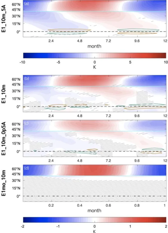
S ENSITIVITY TO THE M IXED L AYER D EPTH

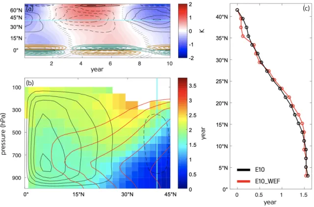
For a shallower mixed layer depth, the response time scale shortens, allowing a higher-frequency extratropical forcing to extend the SST anomalies into the tropics and shift the location of the ITCZ. In other words, the 1-year period is less than the time-scale threshold for the 50-m slab ocean, while the threshold becomes less than one year for the shallower mixed layer. We note that the response time scale shows a distinct deviation from linear characteristics as the depth of the mixed layer becomes smaller (left two circles in Fig. 2.4).

If the depth of the mixed layer is reduced to 2.5 m, the heat capacity of the atmosphere and ocean will be almost the same, indicating a greater responsibility of the fast.

Figure 3.7. Composite across the forcing cycle of zonally averaged response of SST (shading; K) and precipitation (green/brown contour; interval = 5 mm day -1 for E1_10m_5A and 1 mm day -1 for others) of (a) E1_10m_5A, (b) E1_10m, (c) E1_10m_0p5A, and

E FFECT OF R ADIATIVE F EEDBACK ON THE E XTRATROPICS - TO -T ROPICS T ELECONNECTION

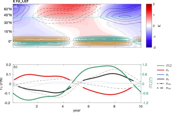
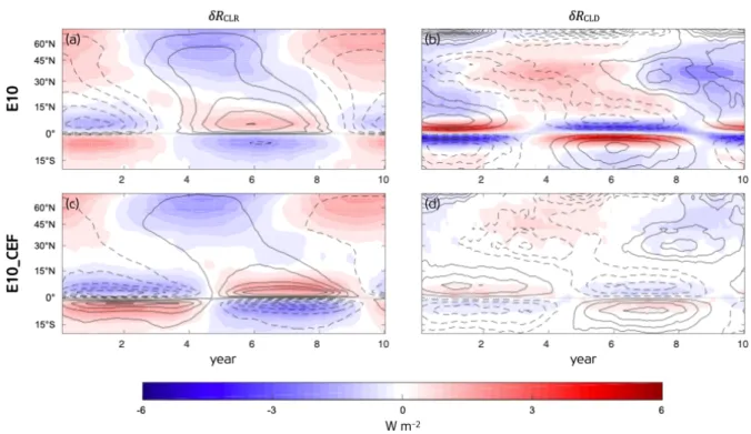
In contrast, in the deep tropics the CRE response acts as a negative feedback to the ITCZ ​​response. In our model, the CRE response in the deep tropics is dominated by the shortwave component over the longwave component (Kang et al. 2014), so that the deep tropical CRE acts as a negative feedback to the ITCZ ​​shift. The analysis of the temporal evolution of the CRE response in E10 suggests that the CRE accelerates the equatorward progression of an extratropical signal while dampening the ITCZ ​​response.

The CRE response in E10_CEF does not completely disappear (Fig.. 1994; Soden et al. 2004), but it is significantly attenuated, allowing us to cleanly examine how the CRE modulates the extratropics-to-tropics teleconnection.

Figure 2.8. Composite across the forcing cycle of zonally averaged response of (left) & &'( (shading; W m -2 ) and specific humidity at 10 m (solid-dashed contour; interval = 0.1 g kg -1 ) and (right) & &') (shading;

S UMMARY AND D ISCUSSION

Where net downward top-of-atmosphere (TOA) radiation 9!"#, net downward surface energy flux .:;, is the angle bracket indicating the vertical average imposed surface flux b Z J K-1 m-2 the specified heat capacity of 50 m oceanic mixed layer. We also employ an idealized thermodynamic-advective model (Takahashi et al. 2007a,b) to demonstrate the importance of mean meridional advection of the MSE anomaly in the lower troposphere for the equatorward propagation of SST. response from the subtropics (i.e., the Hadley circulation terminal). To better understand how the northern extratropical forcing perturbs the southern extratropics, we show in Figure 4.3 the vertical cross section of the zonal mean temperature response composite and 20.67 years after the warming is prescribed poleward of 40°N, which is chosen based on the temporal evolution of the SST anomaly averaged between 3°N-5°N (vertical lines in Fig. 4.1c,d).

The role of water vapor feedback in the response of the ITCZ ​​to asymmetric hemispheric forcing.

T HE T ROPICAL R ESPONSE TO P ERIODIC E XTRATROPICAL T HERMAL

I NTRODUCTION

Therefore, a mechanism controlling SST propagation would explain the sensitivity of extratropical-to-tropical teleconnections. We emphasize that the WES feedback will play a sufficient role in the teleconnection between the extratropics and the tropics to control the magnitude. In the previous chapter, we show a temporal requirement for extratropical-to-tropical teleconnection by considering the transient facet of the energetic framework.

In section 3.2 we again outline general strategies to investigate the sequential mechanism of teleconnection between extratropics and tropics.

M ETHODOLOGY

• I DEALIZED T HERMODYNAMICAL -A DVECTIVE M ODEL

The diffusion coefficient Ä m s-1 is set to best fit the atmospheric energy flux :# from the reference experiment. The clear-sky OLR is parameterized by the least-squares regression of ?2 at each latitude from the reference experiment. The atmospheric mixed layer (AML) is coupled to an oceanic mixed layer (OML) that interacts via sensible (SHF) and latent heat fluxes (LHF).

The AML and OML are respectively governed by the following equations:. by entrainment from the free troposphere, and ?2 is the OML temperature.

Figure 3.1. (left) Time evolution of meridional energy transport predicted by EBM

P ROPAGATION M ECHANISM

• M ID -L ATITUDE E DDY R EGIME
• H ADLEY C ELL R EGIME
• S UBTROPICAL T RANSITION R EGIME

Based on the propagation rate estimated by the slope of the phase line, we identify three different regimes for the teleconnection between extratropics and tropics: the midlatitude eddy regime, the subtropical transition regime, and the Hadley cell regime. The EBM also captures the sensitivity of the magnitude of the extratropical SST variability to the forcing period (Fig. 3.7c). Inside the Hadley cell, the energy transport fluctuation is mainly dominated by the thermodynamic component.

For the experiments with no extratropically forced teleconnection, one half of the forcing period T is indicated by cross symbols.

Figure 3.3. (a) The lag time for which the correlation coefficient is maximized between the tropospheric zonal-mean MSE response and the Qflux forcing as a function of latitude and height (shading; year) in E10

S UMMARY AND D ISCUSSION

We investigate the possibility of pole-to-pole coupling via atmospheric teleconnections by imposing a cyclic surface thermal forcing in the northern extratropics of an ocean model of an aquaplanetary plate. The polar surface warming in the unforced hemisphere reaches 30% of that in the forced hemisphere, inferring an importance of the pole-to-pole connection. Response of the ITCZ ​​to extratropical thermal forcing: Idealized plate-ocean experiments with a GCM.

Fast and slow shifts of the zonally-mean intertropical convergence zone in response to an idealized anthropogenic aerosol.

Figure 3.10. Same as (a) Fig. 2.3, (b) Fig. 3.3a, and (c) Fig. 3.5, but for the E10_WEF experiment

H OW DOES THE HIGH - LATITUDE THERMAL FORCING IN ONE

I NTRODUCTION

In particular, it has been suggested that the polar regions are most effective in inducing remote climate changes (Park et al. 2018). The variability in the Atlantic Meridional Overturning Circulation (AMOC) is thought to be important in formulating the bipolar seesaw (e.g. Stocker and Johnsen 2003; Pedro et al. 2018). Meanwhile, paleoclimate studies of the end of the last glaciation invoke an atmospheric path for the pole-to-pole coupling (e.g. Denton et al. 2010).

However, the observed multi-decadal surface temperature fluctuations at the two poles have recently been shown to be caused by different drivers (e.g. Deser et al. 2020; England 2021).

M ETHODOLOGY

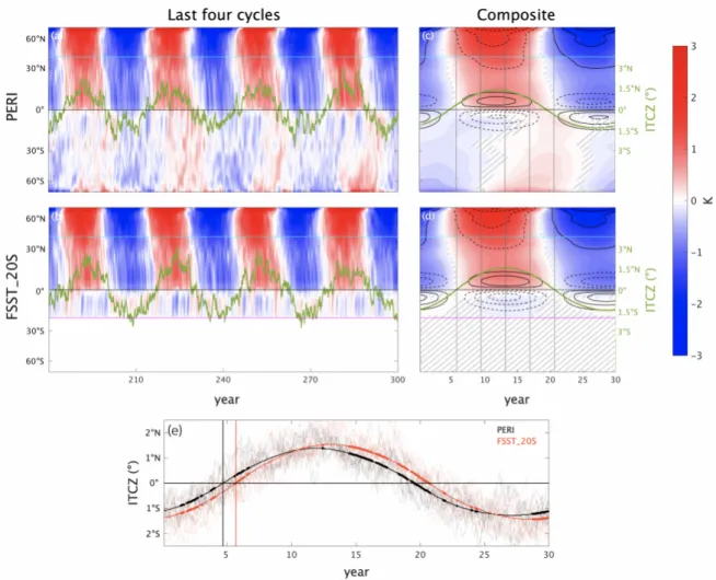
The internal variability in the reference experiment is used to test the statistical significance of the climate response. FSST_20S is also integrated for 330 years with a 30-year rotation, and the composite response is calculated using the last 10 cycles. Considering that the inclusion of the seasonal cycle requires a longer adjustment period, the PSEA is integrated for 450 years, corresponding to 15 cycles.

All the main features we discuss here are robust regardless of the seasonal cycle (contrast Figs. 4.1,3,6 vs 4.8-9).

R ESULT

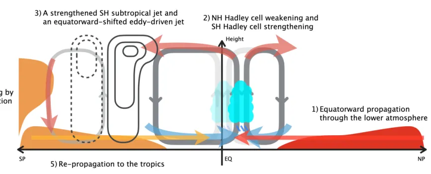
However, the southern high latitudes show a significant SST response, which in turn propagates to the lower latitudes (Fig. 4.1a,c). Compared to PERI, the southern tropical SST response becomes completely out of phase with the northern tropical SST response (Fig. 4.1b,d). The southerly warming response at high latitudes then propagates toward the tropics via the lower troposphere (Fig. 4.3d, e), similar to the near-surface equatorward progression path in the forced NH.

A strengthening of the subtropical jet enhances vertical wind shear, and the increased baroclinicity attracts the eddy-driven jet equatorward (Fig. 4.3b-c,g-h).

Figure 4.1. (a,b) Hovmöller diagram of zonal-mean SST response (shading; K) and ITCZ latitude (green line; °) for the last 4 cycles (i.e., 120 years) and (c,d) composite across the forcing cycle of zonal-mean SST response (shading; K), TOA clear-sky radi

S UMMARY AND D ISCUSSION

동시에 내 연구가 끌리기 시작했습니다. '연구'의 큰 그림을 그릴 수 있었습니다. 하지만 꼭 공부하고 있다고 답할 수 있는 연구자가 되도록 노력하겠습니다.

앞으로도 교수님과 함께하면서 많이 배우고 좋은 연구를 하고 싶습니다.

Figure 4.10. Schematic that depicts how the high-latitude warming in one hemisphere affects the other hemisphere

C ONCLUSION