Optimization of Big-Bore High Pressure High Temperature (HPHT) Wells in Low Pressure Reservoir
by
Alif Aiman Bin Adnan
Dissertation submitted in partial fulfillment of the requirements for the
Bachelor of Engineering (Hons) Petroleum Engineering
MAY20ll
Universiti Teknologi PETRONAS Bandar Seri Iskandar
31750 Tronoh Perak Darul Ridzuan
CERTIFICATION OF APPROVAL
Optimization of Big-Bore High Pressure High Temperature (HPHT) Wells in Low Pressure Reservoir
by
Alif Aiman Bin Adnan
A project dissertation submitted to the Geoscience and Petroleum Engineering Department
Universiti Teknologi PETRONAS in partial fulfillment of the requirement for the
BACHELOR OF ENGINEERING (Hons) PETROLEUM ENGINEERING
Approved by"''· Sonny lrawan
Scni-Jr Lecturer
~~J,;%cience & Petroteum Engineering Oape!ir:tQi1(
tJr;;versiti Teknologi PETRONAS
!3:woar Seri lskantlar, 31750 Tronoh PemK Darul Ridzuan, MALAYSIA
Dr. Sonny Ira wan
':l..~
/trf
2$111Project Supervisor
UNIVERSITI TEKNOLOGI PETRONAS TRONOH, PERAK
May2011
ABSTRACT
Since initial production in early 1990s, the Alpha gas field has been experiencing significant pressure decline. The pressure decline had started to affect the performance of the field; reduced in overall gas production. Subsequently, the extensive pressure decline had caused several wells to collapse due to formation subsidence. The project focused to determine the suitable completion design and casing program for optimum gas recovery from the low pressure environment. The project utilized WellFlo simulation program to compare and analyze the results. Among the identified designs to be simulated are; (1) 10 inch Tubingless Completion (2) Conventional 9-5/8 inch Tubing and (3) Tapered 9-5/8 x 7-5/8 inch Tubing design. The selected design must be able to yield significant increase in gas recovery, extending the producing life of the field and adequate Zonal Isolation to prevent well failure. The 10 inch Tubing1ess Completion had met the required parameters and was selected as the suitable design for the project. The 10 inch Tubing1ess Completion increased gas recovery by 23.15 Percent (%) and extended the producing life of the field up to 16.8 years. In addition, the 7 inch Drill-in Liner provided improved Zonal Isolation between the producing Limestone layer and overlaying Shale structure.
ACKNOWLEDGEMENTS
During this year of finishing up with this project, the assistance, guidance and support had been given by many parties. The author would like to express his utmost gratitude to the Project Supervisor, Dr. Sonny Irawan for the guidance and support given to ensure the progress of the project. In addition, the financial support provided by the Universiti Teknologi PETRONAS (UTP) is highly appreciated as well as the infrastructure provided. The author would like to extend his gratitude to the colleagues who helped, advised, guided and shared the knowledge throughout completing the project. A grateful appreciation is addressed to all who had contributed to the accomplishment of this project, for the constant encouragement and timely help throughout.
TABLE OF CONTENTS
Certification of Approval Certification of Originality Abstract
Acknowledgements Table of Contents List of Figures List of Tables Nomenclature
Chapter 1- Introduction 1.1 Project Background 1.2 Problem Statement 1.3 Objectives
1.4 Scope of Study
1.5 Significance of the Project 1.6 Feasibility of the Project
Chapter 2 -Theory and Literature Review 2.1 Wellbore Completion Design
2.1.1 Tubular Design and Capacity 2.1.2 Tubing Performance Relation (TPR) 2.1.3 Gas Production vs. Time Prediction 2.2 Gas Field Development
2.2.1 Pipeline Flow Calculation 2.2.2 Compressor Station Calculation 2.2.3 Gathering System Calculation 2.2.4 Tubing Flow Calculation 2.2.5 Reservoir Calculation 2.3 Big-Bore Completions
2.4 High Pressure High Temperature (HPHT) Well Condition 2.5 Low Pressure Reservoir
ii iii iv v vi viii
ix
X
1
I 2 2 2 3 3
4 4 4 6 7 8 9 9 9 10 10 II 12 12
2.6.1 Conventional 9-5/8 inch Tubing Completion 2.6.2 10 inch Tubingless Completion
2.6.3 Tapered 9-5/8 x 7-5/8 inch Tubing Completion
Chapter 3- Methodology 3 .I Research Methodology 3.2 Tools and Equipments
3.3 Project Planning- Gantt chart and Key Milestones
Chapter 4 - Results and Discussions 4.1 Reservoir Formation and Structure 4.2 Assumptions and Limitations 4.3 Reservoir Flow Performance 4.4 Completion Design Potential 4.5 Final Design Selection
Chapter 5- Conclusions and Recommendation 5.1 Conclusion
5.2 Future Recommendations
References
Appendix
15 16 17
20 20 25 28
29 29 30 31 35 39
43 43 43
44
46
LIST OF FIGURES
Figure 1: IPR and TPR Plot Figure 2: Typical Production Cycle Figure 3: Total Gas Production System
Figure 4: Typical Monobore Big-Bore Completion Figure 5: Arun Big-Bore Initial Rate Enhancement Figure 6: North Qatar Field Performance
Figure 7: Conventional 9-5/8 inch Tubing Completion Figure 8: 10 inch Tubingless Completion
Figure 9: Tapered 9-5/8" x 7-5/8 inch Tubing Completion Figure 1 0: Optimized Production Cycle
Figure 11: Methodology
Figure 12: WellFlo® General Operation Method Figure 13: Gantt chart and Key Milestones Figure 14: Stratigraphic Model of the reservoir Figure 15: WellFlo Simulation Model
Figure 16: Reservoir Performance for 10 inch Tubingless Figure 17: Reservoir Performance for 9-5/8 inch Tubing Figure 18: Reservoir Performance for Tapered Completion Figure 19: Flow Potential Performance
Figure 20: Operating Point for 1 0 inch Tubingless Figure 21: Operating Point for 9-5/8 inch Tubing Figure 22: Operating Point for Tapered Completion Figure 23: Tapered 9-5/8 x 7-5/8 inch Tubing Figure 24: Gas Flow Rate Depletion Profile Figure 25: Cumulative Gas Production Chart Figure 26: 10 inch Tubingless Completion Design
6 7 8 11 13 14 15 16 17 19 20 27 28 29 30 31 32 33 34 35 36 37 38
39
40 41
LIST OF TABLES
Table 1: Reservoir Data Table 2: Tubing Data
Table 3: Surface Facilities Data Table 4: Compressor Station Data Table 5: Pipeline Data
Table 6: Production Conduit Design Data Table 7: IPR Properties for 10 inch Tubingless Table 8: IPR Properties for 9-5/8 inch Tubing
Table 9: IPR Properties for Tapered 9-5/8 x 7-5/8 inch Tubing
21 21 22 22 22 23 31 32 33
NOMENCLATURE
Quantity Symbol Dimensions
Average Flow Rate QAvg (Mscf/ day)
Difference in Elevation from P wr to P wh H inch
Flowing Bottom Hole Pressure Pwr (lbm/inch2)
Flowing Wellhead Pressure Pwh (lbm/inch2)
Gas Deviation Factor
z
Gas flow rate at Standard Condition Qsc, qsc (Mscf I day)
Gas Specific Gravity G
Moody Friction Factor F
Temperature T (oR)
Tubing Diameter D,d inch
Subscript Symbol Dimensions
Gas Specific Gravity Yg
Gas Viscosity /.1 Cp
Inner Wall Roughness E inch
CHAPTER I INTRODUCTION
1.1 Project Background
The title of the project is 'Optimization of Big Bore HTHP Wells in Low Pressure Reservoir'. The project will be using the completion technology implemented in the Alpha Gas Field in Indonesia. The published paper on the field includes history, applied drilling program, casing plan and the production string configuration used during the development and optimization of the gas field.
The Alpha Gas field was initially developed during the 1970s with the reservoir having High Temperature and High Pressure (HTHP) environment. The first big-bore wells were designed and commissioned in early 1990s to further enhance the field development. The big-bore wells enabled maximum gas-flow rate per well and reduced overall development investments by cutting the number of required wells. Eleven wells were drilled and completed, with flow rates up to 217 MM Scf/Day for each well. The project was considered highly successful [IJ.
As the field continued to be developed, the reservoir pressure in the Alpha field has declined from 7,100 Psi to less than 600 Psi. As a result, 31 wells were lost due to formation subsidence and wellbore collapse. Additional wells were required to meet volume requirements. The new wells were executed under more difficult and challenging environment due to the severe drawdown completion interval [IJ.
The following campaigns were conducted to further exploit the Alpha Gas Fiel4:
• Conversion from 9-5/8 inch conventional production tubing to 10 inch tubingless completions [IJ
• Installation of 7 inch Drill-in Liners across shale collapse zone
• High temperature Underbalanced Drilling (UBD) of the sour gas reservoir
• Rotary drilling through tree components enabling an undamaged completion
1.2 Problem Statement
Continuous production will further reduce the existing reservoir pressure. As reservoir pressure declines, conventional completion string could not provide adequate flow capacity for the gas to flow. This will result in declining gas production rate. To overcome the problem, new completion technology will have to be implemented to continue producing gas from the low pressured reservoir.
1.3 Objectives
• To determine the completion design for optimum gas production
• To determine the casing program for gas production in low pressure reservoir
• To compare the Production V s. Time curves for each completion designs
1.4 Scope of Study
The scope of study is related to conducting production simulations using WellF!o®. The project is divided into three parts: (I) Gather information on Big-Bore completions and conduct theoretical calculations, (2) Construct simulation models using WellF!o® and design the casing program to accommodate production conduit, (3) Generate the Production vs. Time Curves and decide on the completion design which gives the optimum production.
The simulation models are divided into two segments; Static Reservoir Model and Production Conduit Model. Firstly, the Static Reservoir Model is constructed using WellF!o®. The reservoir and fluid properties are entered into the simulation block. The reservoir model will be a constant parameter for the different completion designs.
Secondly, the Production Conduit Model will be developed. The model will consist of three different configurations:
1. 9-5/8 inch Tubing Completion
11. 10 inch Tubingless Completion
111. Tapered 9-5/8 x 7-5/8 inch Tubing Design
hater, casing program will be designed to accommodate the selected production conduit.
The casing design must be able to withstand the force coming from the reservoir matrix and fluid contained within the pore spaces.
Simulations will be conducted on the integrated models which consist of the Static Reservoir Model and Production Conduit Model. A production profile will be generated on each completion designs. The production profile will be illustrated by the Production vs. Time curves which will be used to determine the completion design that generates an optimum gas production.
1.5 Significance of the Project
The project is highly significant for producing gas from low pressure environment.
Optimized production techniques are required to optimally drain the reservoir fluid without causing further damages to the reservoir. In addition, implemented optimized production technology could extend the producing time of the reservoir and delay the investment of well stimulation programs.
1.6 Feasibility of the Project
The project is based on computer simulations to predict the performance of the reservoir depending on the completion program. The project is expected to be completed within 4 months of research period. Positive and implemented outputs are expected to be produced from the project.
CHAPTER2
THEORY AND LITERATURE REVIEW
2.1 Wellbore Completion Design
In addition to the simulation model conducted by WellFlo, theoretical calculations will b€ wndm;t€d to compar€ th€ actual results from the simulation with the results from initial findings. Among the required calculations are:
• Tubular Design and Capacity
• Tubing Performance Relation (TPR)
• Gas Production vs. Time Prediction
2.1.1 Tubular Design and Capacity
The production tubing design and capacity will be the governing variable for the system. The suitable tubing capacity is required to produce the gas at optimum rate while at the same time extending the production plateau of the fi€ld.
The equation for Tubing Capacity calculation is the R.V Smith Equation [9][101.
The equation is used to measure the compatibility of the production tubing to the fluid flow from the reservoir. The Smith Equation is for vertical flow of gas which is similar to Weymouth Equation for horizontal flow [9][101.
- [D5(Pw/~esPwh')s]0.5
Q - 200,000 ( s ) ... (1)
GT Z f H e -1
Where,
s
= 0.375(~~)
The Reynolds Number (NRe) is a ratio of fluid momentum force to viscous shear force. The parameter is used to determine the type of flow presence in the tubing and to calculate the Friction Factor production tubing [9}[10
1. The Reynolds Number equation for natural gas flow is shown below:
NRe =
2::g ···
(2)Relative Roughness (eo) is used to measure the ratio of roughness on the tubing inner wall [9}[101. The equation is given by:
ev =
li ··· E (3)Friction Factor (f) is used for calculating the gas flow rate. We assume the fluid is a Single Phase Gas Flow l91fl01. The equation is given by:
For smooth wall tubing in turbulent flow regime,
f
= 0.0056+ o.;,
2 ••••••••••••••••••••••••••••••••••••••••••••••••••••••••••••••• (4)NRe
For rough wall tubing with fully developed turbulent flow regime,
1 [ 21.25]
{f = 1.14- 2log e0
+
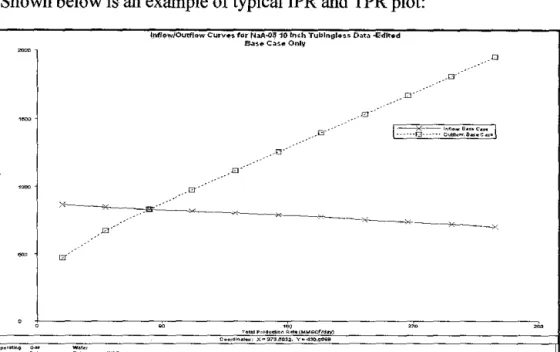
NRe0 .9 ... (5)2.1.2 Tubing Performance Relation (TPR)
In normal practices, the Tubing Performance Relation (TPR) is calculated using Nodal Analysis. For convenience is using the Nodal Analysis technique, the calculations are usually conducted using Bottom Hole (PwJ) as the solution node
[13]
When the Bottom Hole is used as the solution node, the inflow performance is the Well Inflow Performance (IPR) and the outflow performance is the Tubing Performance Relation (TPR); given the end-of-tubing is located above the production zone. The intersection between IPR and TPR curve represents the optimum operating point of the system [I3
J.
Consider the Bottom Hole as the solution node; the TPR is described as below
[13].
6.67 xl0-4 [e5-1]fq 2z 2T2
p wt2
= es + ---::'---''-'---
d5 cos a ··· (6)
Shown below is an example of typical IPR and TPR plot:
lr.fl<>wiOulfl<>w ClltV•~ tor N.>A-<15 10 ln<h Tublrogl•~$ D~t~ -Edlt•d a..~"' c~~ .. Only
o-···_.-···
. .o···
G_ ••• -··
.>:'i···/
'"'
TotoiP•o•ociOoo R _ ( .... SC.,O'>') Coo,Oio"-• X•:m!1l0>2. Y • - . 0 0 0 0
Figure 1: !PR and TPR Plot Pl
.. .o···
o---·· 0
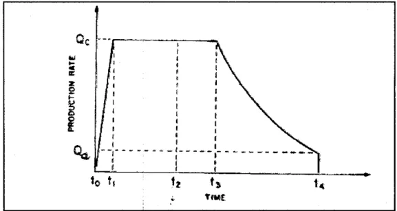
2.1.3 Gas Production vs. Time Prediction
The Production Rate - Time Prediction is used to show the production profile of the producing field. The calculation for the estimation is complex and usually conducted by simulation software for accurate results. Shown below is the general equation used for future production estimations [9l:
T;me = c;_~_~Tf!~_U:~-~-f!: __ Dur~ng Ir_t_~~!""!'!}_
' ... (7)
QAvg
2 2 1637QGTZ!i [ _ _ kt ( -)]
Pwt = P; - log 2 - 3.23
+
0.87 s ... (8)kh ¢JlCtiTw
Attached below is a sample of production cycle curve generated by using theoretical calculations:
I I I I
I I
f 1 I
I I I
- -~-- - - -- = ~ - t- - - - ... - - - - -
' I I
6 I :
Figure 2: Typical Production Cycle [9l
The Production Cycle diagram illustrates the life of the reservoir from initial production to abandonment. It is desirable to have an elongated production plateau before production starts to decline. As production declines, pressure maintenance or artificial lift techniques may be introduced to meet the desired production rate.
2.2 Gas Field Development
Gas reservoir development always directly linked to the market by pipeline; therefore the physical characteristics of the reservoir could not predict the best depletion pattern because the market must be able to accept the gas [91. The design of an optimum development plan for natural gas field depends on the typical characteristics of the producing field as well as the markets to be served by the field [91.
However, basic field parameters; (1) total natural gas reserves (2) well productivity (3) dependence of production rate on pipeline pressure (4) depletion of natural gas reserves, are required prior to designing the development scheme of the field [91.
Key elements that affect the total gas production system are stated below [lJJ:
1. Flow through the Reservoir
ii. Flow through the Production String
iii. Flow through the Field Gathering System and Processing Equipment tv. The Compressing of the Gas
v. Flow through the Auxiliary Pipeline to the point of sale
I MAI!KET
i
jI
I I
INFlOW PERFORMANCEFigure 3: Total Gas Production System [l3J
2.2.1Pipeline Flow Calculation
The calculation uses Panhandle equation to determine the pressure required at the discharge point of the compressor [I3J.
1.07881 2 2 0.5394 0.4606
Q = 435.87 (E)
(Tb)
(Pl - P2 )(.!:.)
(D)Z.6182 .•..•.. (9)Pb T.L.Z G
2.2.2 Compressor Station Calculation
The calculation utilizes adiabatic compression equation to determine the Suction Pressure (Psuc) at the intake of the compressor [I3J.
HP ( K )
[(pd. )k~l
]- - : -
1 = 0.08578 - (Tsuc)(Zsuc) _____£ - 1 ... (10)
MMsc d k-1 Psuc
_ _ (HP /MMscfd)(Q)
BliP= E •••••••••••••••••••••••••••••••••••••••••••••••••••••••••••••••••••• (!!)
2.2.3 Gathering System Calculation
The gathering system consists of multiple pipelines that linked to a single gathering station from different producing wells. The calculation uses Weymouth to find the Wellhead Pressure (P if) of a single well [!31.
Q =
KjPt/- Psu/ ...
(12)2.2.4 Tubing Flow Calculation
The calculation uses correlations for vertical flow such as Hagedorn and Brown method to find the Flowing Bottom-Hole Pressure (P,,1) [131.
[DS(p 2 wf - e · s p. tf 2) ]0.5 s
Q = 200,000 ( s ) ... (13)
y9 .T.Z.f.L e - 1
0.0375(y9)(L)
s
= T.Z ··· (14)2.2.5 Reservoir Calculation
The calculation uses the Well Spacing Coefficient ( Cavg) from the well test analysis. The Flowing Bottom-Hole Pressure (Pwt) from the reservoir side is matched to the pressure from surface back-calculations. The difference is the value should not exceed 3 Psia [lJJ.
Q = CaviPR 2 - Pw/r ... (15)
The pressure drop must be considered in each of the components in the production system. The restrictions presence in the components must be within the tolerance limit to allow gas to flow to the point of sale. Excess pressure drop will cause gas to accumulate and cause pressure build up at the bottom of the well. Other problems related to hydrates formation may occurred as the pressure increases in the well [131.
2.3 Big-Bore Completions
The objective of Big-Bore completions is to reduce the life cycle costs of developing prolific, high profile gas reservoirs. Completions that use 6-5/8 inch or bigger tubular design are considered as Big-Bore completions. The design can significantly reduce both operating and capital expenses and increase the net present value of hydrocarbon assets.
[14]
,j·
';:
1~·-..
f..
tj
Figure 4: Typical Monobore Big-Bore Completion [141
The larger production conduit provides increased flow area, while the monobore scheme reduces flow restrictions. Other benefits include [I6l:
• Eliminate gas turbulence areas lllld restrictions on production
• Earlier Return oflnvestment (ROI)
• Exploitation of the reservoir through fewer wells
• Lower long-term operating expenses from quicker depletion of the reservoir
• Lower topsides and maintenance expenses
2.4 High Pressure High Temperature (HPHT) Well Condition
A High Pressure High Temperature (HPHT) wells are hotter and more pressurized than typical wells. In HPHT wells, the bottomhole temperature or temperature at Total Depth (TD) is higher than 300 degree Fahrenheit (149 degree Celsius) and pore pressure reaching at least 0.08 Psi per foot l17l.
Typical HPHT reservoirs are found in the North Sea, deepwater of the Gulf of Mexico and China. Currently the number of well drilled and completed with HPHT characteristics are still low but the number is increasing [171•
By nature, high pressure fields contain more hydrocarbons than those with normal conditions. As long as the fields boast enough reservoirs, the development of HPHT wells is economical. In addition, operating at HPHT conditions is extremely dangerous and increase risks to drilling, completion and work-over activities. Strict operating procedures are implemented to ensure the safety of HPHT operations [171.
2.5 Low Pressure Reservoir
Low pressure reservoir is considered as reservoir having pressure less than 1000 Psi.
Low pressure environment usually occurred when the reservoir's natural drive or energy rapidly declines after several years of production [11• The reservoir's energy usually originated from:
• Strong aquifer support from bottom shale formation or water-bearing zone
• Energy from dissolved Free Gas or dissolved Solution Gas
• Energy from the compressed rock matrix and formation fluid
• Energy from gravity drainage
After producing for several years under its own natural drive, pressure maintenance scheme such as gas or water injection is usually implemented to sustain production.
Significant enhancement on the completion design would made production more
2.6 Literature Review
The objectives of the project are: (I) to determine completion design for optimum gas production, (2) to determine the casing design for producing in low pressure reservoir, (3) to compare the Production vs. Time curves for each completion designs.
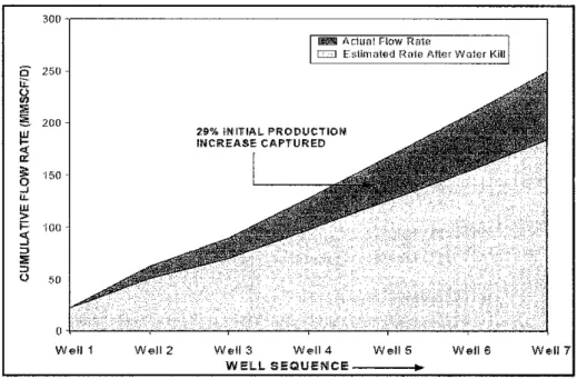
The completion technologies applied in the project were based on the gas development projects performed in the Arun field in Indonesia and the North Field in Qatar. Both of the fields were producing for several years and major re-development programs were implemented to further exploit the two fields. The Arun gas field in Indonesia had adopted the 1 0-inch Tubingless Completions on the re-development campaign to construct seven new wells in 2002. The implementation of the completion design had increased the initial production up to 29% [IJ.
300
111!11 A c:lual Flow Rate
c::=::J E>11imated Ruie After Water Kill
29% I·N·ITIAL PRODLIC1'10N INCREASE CAPT'UR:ED
0-~~--~--~---r~~~~~~~~~~~~~~
Well1 Well2 WeH3 We-114 Well5 Wel16 Well7
WELL SEQUENCE
Figure 5: Arun Big-Bore Initial Rate Enhancement [ll
The North Field in Qatar had adopted the Tapered 9-518 t 7-5/8 Tubing x 7-inch Uner design on eight new wells to produce gas at 200 MM scfd. The design had resulted: (I) minimizing the overall development cost by reducing the number of wells to be drilled.
(2) enable production plateau to be extended by having higher nowing wellhead P 121
pressure, wh .
Figure 6: North Qatar Field Performance '21
The implementation of the two designs in respective locations had proven significant increase in production volume as well as reducing the overall development cost and time.
The completion designs to be simulated in the projects are taken from the projects in Indonesia and Qatar. The three types of completions are explained in the following parts:
2.6.1 Conventional 9-5/8 inch Tubing Completion
The design incorporates the use of 9-5/8 inch Production Tubing from the surface (0 ft) to the top of the 10 inch Liner. The productive zones will be completed Open-Hole with the hole having 8-112 inch Diameter. This enables the well to have total production conduit of 9-5/8 x 10 x 8-112 inch in Diameter. The casing program uses 30 inch Driven Conductor followed by 20 inch and 13-3/8 inch Steel Casing to isolate the formation. Below the 13-3/8 inch Steel Casing is the 10 inch Liner followed by Open-Hole completion with 8-1/2 inch Diameter into the productive zones [lJ.
Attached below is the completion schematic to further describe the design:
'0"
Dn~enJ
! ~2tl"
:;
"
c
~
9-5/8" Tttbwg
rJ •. l/8 .. . - - - -
w·-Lirm
8-l
/~·-·Open Hole~ J
Figure 7: Conventional 9-5/8 inch Tubing Completion [I]
2.6.2 10 inch Tubingless Completion
The design uses 10 inch Tubingless conduit from the surface (0 ft) to the top of productive layer. 7 inch Drill-in Liner will be installed at the bottom of the Tubingless conduit to enable drilling operations into the productive carbonate reservoir. The production zone will be completed Open-Hole with the hole having 5-5/8 inch Diameter. This enables the production conduit to have total volume of 5-5/8 x 7 x 10 inches in Diameter. The Casing Program is similar to the Conventional 9-5/8 inch Tubing Completion with the addition of the Drill-in Liner and smaller Open-Hole completion [IJ.
Attached below is the 10 inch Tubingless Completion diagram:
Jo:.~
Dtirttl i
..
-
20"'
• ' ;
,.
JJ.Jii' ...
lO'FuiJSJnug
~
IT Drilhrlg LlllH
~
J
5-5•S0p<nHol</ •
"----
Figure 8: 10 inch Tubingless Completion [IJ
2.6.3 Tapered 9-5/8 x 7-5/8 inch Tubing x 7 inch Liner Completion
The design uses Tapered 9-5/8 x 7-5/8 inch Tubing. The Production Tubing connects to the 7 inch Liner which penetrates through the productive rock layer.
The design is different compared to the Conventional 9-5/8" Completion and I 0"
Tubingless Completion. The Tapered Completion design has a cased productive zone rather than having Open-Hole completion. The tapered design allows gas expansion along the production conduit as the gas pressure is reduced. The Casing Program for the Tapered Completion also differs with the previous two completions. The casing program uses 30 inch Drive Conductor followed by 18- 5/8 inch and 13-3/8 inch Steel Casing. The lower section of the 13-3/8 inch Casing is completed with 9-5/8 inch Liner and 7 inch Liner will penetrates the producing zone [21 .
Attached is the diagram for the Tapered 9-5/8 x 7-5/8 inch Tubing Completion:
30"411
! ~9-5/8"
scssv
, I
18-5/8' <ill .
..
1-9-518' x7.SI8"
~~
Tubing13-318' AI
fs18" Liner A ,~
7" Liner
... ...
Figure 9: Tapered 9-5/8 x 7-518 inch Tubing Completion [21
The Production Conduit Model will be based on the three completion designs. The Production Conduit Model will be integrated with the Static Reservoir Model to initiate simulation. Simulation will be conducted on the integrated model to determine the design which results the optimum gas production. The optimum production can be described as:
• Having extended production plateau
• Having longer production time
• Having low differential pressure (M) between the bottom of the well and wellhead node
The second objective is to design the casing program to accommodate the production conduit. Different completion design would have different casing configuration due to the size of the production conduit. For example, the Conventional 9-5/8 inches Tubing would have the 30 inch Driven Conductor followed by 20 inch Conductor Casing, 13- 3/8 inch Surface Casing and 10 inch Liner [IJ. The casing design will determine the size of hole to be drilled. The function of the casing program includes:
• To protect the inner production tubing from compressive force from the formation
• To prevent formation collapse or subsidence
• To prevent crossflows between water bearing zone and productive hydrocarbon zone
• To isolate different formation layers (shale, limestone, sandstone)
The casing used will have to bear the external compressive force and the internal burst energy acting on the casing wall. Materials such as 129#X -52 Steel and L-80 Steel will be used extensively in manufacturing the casing. Each casing connections would have a gas tight premium connection to avoid gas from escaping through the casing's micro- annulus gaps [IJ.
In field practices, the annulus between the casing and the formation will be cemented.
The cement will provide better Zonal Isolation in addition to the casing program. Zonal Isolation is important to prevent fluid escaping to the surface, mixing of unwanted fluids and formation collapse or subsidence 121.
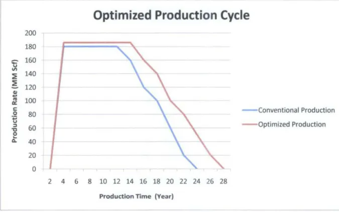
The third objective is to compare the Production vs. Time curves for each completion designs. The curve will be generated using WeliFio®. The curve should be achieved after simulation is conducted on the integrated model. The curve will illustrate which design yields the optimum rate. The curve will be analyzed based on two main parameters: (1) total production years, (2) extension of production plateau before decline. Attached below is a sample of optimized production cycle [JI:
f Optimized Production Cycle
200 180
£'
Ill 160~ 140
~ 120
- ...
Qlnl 100
a::
c:: 0 80
'B :s 60
"C
Conventional Production Optimized Production
...
0~ 40
20 0
2 4 6 8 10 12 14 16 18 20 22 24 26 28
Production Time (Year)
Figure 10: Optimized Production Cycle 131
CHAPTER3
METHODOLOGY
3.1 Research Methodology
Construct Static Reservoir Model with constant parameters; Reservoir Pressure, Porosity, Permeability, Gas Density, Skin Factor, Temperature
Construct Production Conduit Model with different configurations:
• Conventional 9-5/8" Tubing
• I 0" Tubingless Completion
• Tapered 9-5/8" x 7-5/8" Tubing
Integrate Static Reservoir Model with Production Conduit Model.
Commence simulation on the integrated model to detennine the design which
yields optimum production
Generate Production Cycle graph; Production Rate vs. Time
Expected Production Profile
P l ' • f JD J:l J.' :• f 1V u H H ,f l(l
... w..._ ... «.-•t~
Decide on design which yields optimum production
I I I I I -----~
I I I I I I I
Pipeline Calculation
G )
10788l(p l_ p 2)0.5394(1)0.4606
Q = 435.87 (£) 2. _J - ' - (D)2.6182
~ Tl.Z c
---------------~-----------
_____________________ t 1 ________________ _
Compressor Calculation
__!!!__ =
0.08578(~)
{T. )(Z )[f!..d•s)-;J - 1]
MMufd k-1 sue sur \Psuc
BHP = (HP MMscfd)(Q) E
---- --- --- --- ---,- -- --- ___ _ _____ _ _____ _ _____ i __ _ _ _____ _ ______ _
Gathering System Calculation
--- --- --- --- r----
I--- -- --- -
~
Tubing Flow Calculation
Q = 200,000 D P,,l - e .Pet- s
[
" ( 2 s ~)
] 0.5
y0 .T.Z.f.L(eS-~)
S = 0.0375(y11)(L) T.Z
--- -- ---.----
1--- ---
----------~-------------
1 I I I I
Reservoir Calculation
( z 2)n
Q = Cavo PR - P .... .,,.
'--- --- --- --- --- ---
Design and integrate the Casing program with the Tubing design
Reservoir Data
Average Reservoir Pressure, P, 875 psia Average Reservoir Temperature, T, 350°F I 810°R
Average Reservoir Depth, Z 10,200 ft (TVD)
Average Net Payzone Thickness 180ft
Average Porosity, 0 18%
Average Permeability, k 320mD
Wellbore Radius, rw 5.625 inch
External Radius, re 1500 ft
Drainage Area, AI 7. 069 X 10° fi"
Darcy Flow Coefficient, B 146509.8 MMscfd
Fetkovich Coefficient 0.0005
Average Water Saturation 10.7%
Formation Volume Factor, Bo 1.32
Gas API Gravity 86 °API
Gas Specific Gravity, y0 0.65
Gas Viscosity, fig 0.25 cp
Number of Wells, N 5
Well Spacing Coefficient, Cavg 0.00742 MMscfd/psia
n-coefficient 0.75
Pseodo"Critical Pressure, P pc 671 psia Pseodo-Critical Temperature, T pc 370°R
Table 1. Reservozr Data [!Jl2J
Tubing Data
Tubing Length, Ltubing 10,000 ft (TVD)
Average Tubing Temperature, T 100°F I 560°R
Compressibility factor, z 0.90
Tubing Diameter, D Depends on types of completion
Friction factor,/ 0.0144
Surface Facilities Data
Ratio of flowrate and pressure, K 0.763 x 10 scfdlpsia Table 3: Surface Facilities Data
Compressor Data
Operating Limit, BHP 20,000HP
Efficiency, E 0.80
k-factor 1.25
Suction Temperature, Tsuc 60°F I 520°R
Compressibility factor, Zsuc 1.0
, [IJLLJ
Table 4. Compressor Data
Pipeline Data
Pipe Length, Lpipe 120 miles
Pipe Diameter, D 13 inch
Output Pressure, PL 200 psia
Average Temperature, T 70°F I 530°R
Efficiency, E 0.92
' '
Base Pressure, Pb 14.73 psia
Base Temperature, Tb 60"F I 520"R Table 5. P1pelzne Data [IJ[LJ
Production Conduit Model Data
Conventional 9-5/8
•
Productive layer ISInch Completion completed Open-Hole \0
Dri~-?~~ i ~
Tubing with 8-1/2" hole diameter
:!{1"
•
Production conduit IS-
'completed with 1 0" Liner
'
connected to 9-5/8" 9-s .. s·· Tubmg
Tubing to surface
Jl.;.,---
JW- Linfr
S-1'2-''0ilCnHote__..:J l . - - -
10 Inch Tubingless
•
Productive layer ISw I Completion completed Open-Hole with Drir;11~ · ~
5-5/8" hole diameter 2 0 - -
~~
•
Production conduit uses ',
10" Full String Tubing
' from top of production
zone to surface
ll-;3~
•
Incorporates the use of 7"Drill-In Liner to penetrate
J(l .. foiiStrmg
~
'30 ft into production zone
i
T Drillm~ Lintr -
5-5-S''OpeoHole/
Tapered 9-5/8 Inch
•
The productive zone IS31)'.4
~x 7-5/8 Inch Tubing completed with 7" Liner 9~18"
scssv
with perforations
•
The production conduituses tapered 9-5/8" X 1S.QIS' ~
..
7-5/8" Tubing connected ! r--..9-518' x7-51S' Tubing
to the top ofT' Liner
'
13-318' J i L
.Q/8" Liner .oil
..
7' Liner
' ..
' [1][2][3]
Table 6. Productzon Condwt Data
3.2 Tools and Equipments
In the project, WeliFlo® software will be used to conduct the gas production simulation with different completion configuration.
WeliFlo® is a Nodal Analysis program. Its function is to analyse the behaviour of petroleum fluids in wells. The behaviour is modelled in terms of the pressure and temperature of the fluids, as a function of flowrate and fluid properties. The program takes as its input a description of the reservoir, well completion and the surface equipment. This is combined with fluid properties data. The program then performs calculations to determine the pressure and temperature of the fluids. Different modes of operation can be employed to either solve the flowrate given controlling pressures (typically done for deliverability calculations) or solving for pressure drops given measured flowrates (typically done for diagnostic calculations) [121.
WellFlo® calculations are based on Nodal Analysis. There are two main types of Nodal Analysis; (1) determination of flowrates from pressures [121, (2) determination of pressures from flowrates [121. Determination of flowrates is concerned with deliverability applications while the determination of pressures is concerned with monitoring or diagnostic applications [121.
Deliverability Applications
1. Calculating the flow potential ( deliverability) of a well
Uses techniques to determine operating point- whereby pressures at the node in the system are calculated from a range of flowrates. Only one flowrate will give the same pressure at the solution node calculated in both directions (intersection of IPR and TPR curves) [121.
2, Designing the completion of a well
Enabled the calculations of deliverability as a function of different sizes of tubing or different perforations. This allows the optimum completion is chosen. Design facilities also include valve positioning, valve settings and ESP selections [121 .
3. Modelling the sensitivity of a well design
Reflects the different factors which may affect the production system such as water encroachment or decreasing reservoir pressure. This may refme the design of well completion components. Such sensitivities may pertain to the reservoir, well, surface facilities or operating conditions [121.
Diagnostic Applications
1. Comparison of measured data with calculated data
It can be used for different purposes such as evaluating the best flow correlation within WellFlo®, evaluating match parameters (pipe roughness) or determining if the well is behaving as expected performance [121.
2. Monitoring well performance
To predict reservoir pressure from measured surface pressure and flowrate.
This would enable users to see if the system is behaving as predicted even if all parameters are not measured at the same time [121.
3. For designing production system
Mainly used to calculate the pressure drop or drawdown in a system. This will determine whether fluids are able to flow in the system. Optional facilities are also available to select ESPs and motors for the production system [l2J.
The following part will describe the required information to be entered into Wel!Flo®.
Setting Up a Well and Reservoir Description.
Particular model such as PVT, IPR, vertical lift, temperature and choke calculation need to be selected.
Data Preparation
Performed via Graphical Editor which allow user to select well and surface components from drop-down list.
Analysis
Performed via several options and can be selected from the drop-down menu
Output
To save complete record of the - calculated results and input data to file
' '
.
' Reservoir data ' '
.
---~ Well completion design Surface facilities
'
.
' '
'
.
' Fluid properties data
'---
r---
0
: • Reservoir model for IPR ' '
---...:
'.
computations Reservoir fluid PVT' : • Sensitivities I correlations ' • Gas lift svstem or ESP
1--- r---, ' '
.
---
...
': .
Pressure Drop calculation Operating Point determination----, ' ' ' '
' '
: • Incorporate multiple : sensitivities
' : • Apply flow, choke and temperature correlations
• Gas Lift modelling
• ESP performance
r---,
' '
: • Performance summary 1
' '
L - - - -"': • Graphical report
' ' • Report listing : ' ~---' '
Figure 12: Wel!Flo® General Operation Method [t2J
3.3 Project Planning- Gantt chart and Key Milestones
Final Year Project (FYP-1) Final Year Project (FYP-2)
Activity I Week 1 2 ~. 4 5 6 7 8 9 10 11 12 13 14 1 2 .3 4 5 6 7 8 9 10 11 12 13 14 Gather infurmation regarding Big-Bore WeDs
optimization
Conduct initial theoretical calculation regarding gas production and tnbing design using Deliverability Analysis
Construct Static Reservoir Model with constant furmation and fluid properties Construct Production Conduit Model with 3 diffurent completions
Integrate both Models and commence simulation
Generate Production Cycle Curve;
Produced Rate vs. Time fur each completion designs
Decide which design yields optimum production over time
Design Casing Progarn to accommodate selected design
Integrate Production Conduit with Casing Program
Final Year Project (FYP-1) Final Year Project (FYP-2)
Milestones I Week 1 2 3 4 5 6 7 8 9 .10-12 13 14 11 2 3 4 5 6 7 8 9 10 11 12 13 14 Completion of Static Reservoir Model
•
Completion of Production Conduit Model
~
Completion of dynamic simulation Completion of Production Cycle profile Completion of Casing Program
CHAPTER4
RESULTS AND DISCUSSIONS
4.1 Reservoir Formation and Structure
The gas production zone is from the K-30 Limestone formation at average depth approximately 10,200 feet (TVD). The Limestone reservoir consists of consolidated matrix structure which prevents any sand or carbonate material production during the depletion of the dry gas reserves. Good porosity and permeability is obtained from the reservoir with average porosity and permeability at 18% and 320 mD, respectively. The critical aspect of the Limestone reservoir is that the payzone is overlaid by over-
pressured water bearing formation and highly compacted shale structure flf.
The presence of these two elements had resulted abnormally pressured condition which continues to compress the Limestone reservoir. The pressure gradient across the Shale structure is around 0.039 Psi/ft. The Limestone reservoir is expected to experience deformation or damage when the reservoir pressure depletes to 400 Psia. The overburden stress from the water bearing zone and Shale structure will cause the Limestone reservoir to compacts and collapses '11.
Upper Formation
Overpressured water zone
Shale Format1on
K-30 Layer
P<'t~ Pn.-... ... urc 4pp,;l
I I I I I I I I I I I I I I I I I I I I I
I I I I
I I I I
I I I I
I I I I
I I I I
'
4.2 Assumptions and Limitations
The simulation only focuses on the types of completion to optimize gas recovery. Other parameters such as gathering lines, compressor stations and transmission lines will not be discussed in the paper. Hence, several assumptions and limitations are set to meet the focus of the project. Among the matters are:
1. Reservoir pressure is simulated only to 450 Psia to avoid the effects of reservoir damage to the total production system.
2. Any change is reservoir rock and fluid properties are neglected.
3. Water-cut is not present in the system.
4. No heat loss is considered in the total production system (adiabatic operations).
5. The gathering lines at the surface are represented by the K -coefficient which is at 0.763 x 10⁶ Scfd!Psia.
6. The compressor station is assumed as a single unit having 20,000 HP.
7. Change in flow regime within the transmission lines is neglected.
8. Pressure at end oftransmission lines are set at 200 Psia
Gathering Lines
r----...;_----1 Compressor Station
Cornpliction Conduit
K-30 Lirnesto11c Reservoir
Transmission Li11cs
Figure 15: Wel!Flo Simulation model
....
1li s
..
~ !!!
"-
"'
c
l >;::
..
0.t:;
!
4.3 Reservoir Flow Performance
The reservoir performance is defmed as the Inflow Performance Relation (IPR). The IPR measures the potential of the reservoir at given average reservoir pressure. Shown below
are the IPR curves for each of the completion designs; 10 inch Tubingless Completion, 9-518 inch Tubing and Tapered 9-518 x 7-5/8 inch Production Tubing.
Reservoir Perform~nce for N~-0510 inch Tubingless D~t~ -Edited
1000
7!!0
1!00
1!00 7!!0
T~l Oa P,.dvdion R.te (MMSCF/d.y)
RHttwe~lf P•lform.1n01
I
~ Sud pr.-ur•
1000
UJ•r IPR Wodel Pl.ytr AOF B F
psu WMSCF/da. psQ/~Msctfday) ptQ/~t.tldfd~
K-30 S•nd Norm Pstudo PtttRirt 870.000 V2V.e20 643620Q8 0 AOr(oomp.,o)
Figure 16: Reservoir Performance for I 0 inch Tubingless completion
1 0 inch Tubingless Completion
Wellbore Diameter 5.625 inch (Open Hole)
Absolute Open Flow (AOF) 929.629 MMscfd
Initial Reservoir Pressure 875 Psia
Table 7: IPR properties of 10 inch Tubingless completion
1000
751
..
1ll .s .,
~ !
0..
"'
-
c
l L;: .,
0 "'
~
Uyol
N)f(oompnrtt)
Reservoir Perfonrt3nct for N3A~5 9-5-8 Inch Completion D3t3.Cdlted
300 1100 1100
hUI G• Pto4.vdl•• Rite (WWSCfl4'l')
Pl.,., N)f
,.., WWSCF/foy
876.000 1011021!0
Figure 1 7: Reservoir Performance curve for 9-518 inch Tubing
Conventional 9-5/8 inch Tubing Completion
Wellbore Diameter 8.5 inch (Open Hole)
Absolute Open Flow (AOF) I 096.266 MMscfd
Jnjtial Reservoir Pressure 875 Psia
Table 8: IPR properties of9-518 inch Tubing
Rtstrvolt Ptrform•noe K-30 S•nd ptttiUtfi
1200
1000
7~
'"
111
8 .,
~ .,
.t
"' eoo
c:
l 0
;;: .,
.c: 0
8 i
0 0
l..oy<r
AOF(oomposrto)
IPR Yodtf Pl.t)l•t psi•
875.000
Reservoir Perform~nct for N~.()5 T ~pered Completion O;n~-Edlted
llO
AOF WWSCrld•y
344.873
Jq4.873
180
Toll! 0• Produdion Rlllo (WWSCrld'Jl Coonlln•ta 1.• 3741711'1, Y• ·208 7542
270
Figure 18: Reservoir Performance curve for Tapered Completion
Tapered 9-5/8 x 7-5/8 inch Production Tubing
Wellbore Diameter 7 inch (Cased Hole)
Absolute Open Flow (AOF) 344.873 MMscfd
Initial Reservoir Pressure 875 Psia Table 9: IPR properties Tapered Completion
Rtstwoft PtrfonnJnct
~30 SJnd pttSUtt
In general, having larger wellbore diameter would increase the flow potential of the reservoir. The increase in flow potential is described in the Absolute Open Flow (AOF) value. The AOF value is obtained when the reservoir pressure is equal to zero or at atmospheric condition; 14.73 Psia. This condition is only achievable theoretically and not in real operating environment 191!101.
Larger wellbore diameter would increase the effective drainage contact area, which permits higher flow potential. In addition, the flow potential is also affected by the productive zone completion method whether completed Open Hole or Cased Hole.
As shown above, when the productive zone is completed Open Hole, the flow potential of the reservoir increases by 62.6%. This is because the Open Hole completion allows greater exposed drainage area II]. Cased Hole completion has rather restricted exposed drainage area which only achievable when perforated 121. For gas production, Open Hole completion is preferred for greater flow potential from the reservoir's perspective.
The flow potential increases by 15.2% when the Open Hole completion is increased from 5.625 inch to 8.5 inch. Larger diameter would increase the exposed area thus increasing flow potential. The performance of the three completions is iiJustrated below:
Flow Potential Performance
1200
~ 1000 1096.266
0 !3.
~ 0 800
~ c: • 10 INCH TUBINGLESS
Ql 600
a. TAPERED COMPLETION
0
Ql 400
..
::s 9-5/8 INCH TUBING0 "'
.a ~ 200
0
"'
0 0 0 0 0
... ~ 0 :1
If
..
c. c:
.D
"
t- .!; £
0
..
10 11 5 •! ~
D-
4.4 Completion Design Potential
The tubular performance of the system is shown in the Tubular Performance Relation (TPR) curve. The intersection between the IPR and TPR curve will be the optimum operating point of the system. Results for the three completions are shown below:
10 inch Tubingless Completion
lnftowiOutftow Curves for N3A..OII10 Inch Tublngl•ss 03t3 -Edit•d 83s• C3s• Only
2000
.0
a
.El
1510 0
.cr ,_ E3
o-•-c-
lnft_B_C_I
[]
.o·


![Figure 7: Conventional 9-5/8 inch Tubing Completion [I]](https://thumb-ap.123doks.com/thumbv2/azpdforg/11107565.0/24.863.302.569.476.987/figure-7-conventional-9-inch-tubing-completion-i.webp)