of the requirements

Dynamic Simulation of Quadruple Tank System

by

Asyraf bin Maskan

Dissertation submitted in partial fulfillment of the requirements for the

Bachelor of Engineering (Hons) (Chemical Engineering)

SEPTEMBER 2011

Universiti Teknologi PETRONAS Bandar Seri Iskandar

31750 Tronoh Perak Darul Ridzuan

Approved by,

CERTIFICATION OF APPROVAL

Dynamic Simulation of Quadruple Tank System

by

Asyraf bin Maskan

A project dissertation submitted to the Chemical Engineering Programme

Universiti Teknologi PETRONAS in partial fulfillment of the requirement for the

BACHELOR OF ENGINEERING (Hons) (CHEMICAL ENGINEERING)

(riRM\RAMASAMY) ~~

UNIVERSITI TEKNOLOGI PETRONAS TRONOH, PERAK

September 2011

CERTIFICATION OF ORIGINALITY

This is to certify that I am responsible for the work submitted in this project, that the original work is my own except as specified in the references and acknowledgements, and that the original work contained herein have not been undertaken or done by unspecified sources or persons.

(ASYRAF BIN MASKAN)

ABSTRACT

The problem of estimating state of dynamical system from only input and output measurement remain always an important field in the system theory. In fact, observers play a key roles during monitoring of process, a there are shown an essential component in many control application such as output regulation. Ahhough the theories and applications for linear systems are well developed, development of observers for nonlinear system still provides an open area for research. Quadruple tank system and its mathematical model with typical parameters value will be collected from the reflected real system of quadruple tank. Dynamics simulation will be performed and through the MATLAB® enhancement. Various input changes take part. The result of the simulation will be analyzed and reported.

TABLE OF CONTENTS

TITLE PAGE

CERTIFICATION OF APPROVAL CERTIFICATION OF ORIGINALITY ABSTRACT.

TABLE OF CONTENTS

LIST OF TABLE AND FIGURE CHAPTER !:INTRODUCTION 1.1 Background of study 1.2 Problem Statement

1.2.1 Problem Identification 1.2.2 Significant of the project 1.3 Objectives

I

11 111 IV

v 2 4 4 4 4 5 5

1.4 Scope of study 5

1.4.1 Dynamic mathematical model of quadruple tank system 5 1.4.2 Input and output regulations of the system 6

CHAPTER 2:LITERATURE REVIEW 8

2.1 Process Model.

2.2 Current Process Model Simulation Application 2.2.1 Quadruple tank simulation

8 10 11 2.2.2 Development in multivariable control simulation 12

2.2.2 Easy-Java simulations fundaniental 13

CHAPTER 3:METHODOLOGY 14

3.1 Methodology . 14

3.2 Project activities 15

3.2.1 Process model derivation 3.2.2 Software set up

3.2.3 Simulation initial test

3.2.4 Generation oflnput-Output Data 3.2.5 Validation

3.2.6 Data analysis

CHAPTER 4: RESULTS AND DISCUSSION

15 16 17 18 20 20 21

4.1 Results.

4.1.1 Steady states 4.1.2 Valve constant

4.1.3 Water tanks hole areas and pump constants 4 .1. 4 Deviation

4.1.5 Parameters values and final model 4 .1. 6 Validation

CHAPTER 5: CONCLUSION AND RECOMMENDATIONS 5.1 Conclusion

5.2 Recommendations REFERENCES

APPENDICES

LIST OF TABLE

21 21 23 25 26 27 29 30 30 31 32 33-42

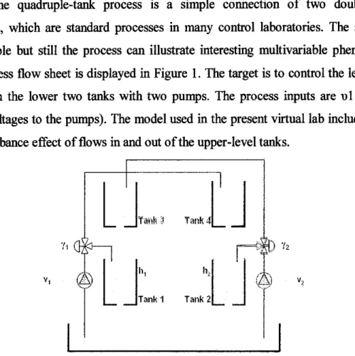
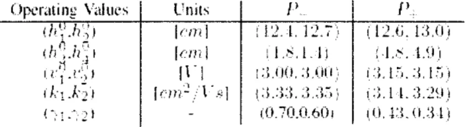
Table 1.0: Parameter value for quadruple tank system 10 Table 2.0: Operating parameter for minimum (P-) and non-minimum (P+)

phases 10

Table 3.0: ODE's Function in Matlab 15

LIST OF FIGURE Figure 1.0:

Figure 2.0:

Figure 3.0:

Figure 4.0:

Figure 5.0:

Figure 6.0:

Figure 7.0:

Figure 8.0:

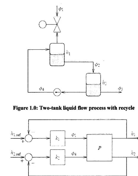
Two-tank liquid flow process with recycle

Two-loop feedback control of the two-tank liquid flow Schematic of the quadruple-tank process

Simulation results for steady state condition.

Results of minimum phase zero configurations.

Results of non-minimum phase zero configurations

Simulation results. Process model with minimum phase zero Deviation oflevel Tank 1 and Tank 2 during 470 seconds Figure 9.0: Real behavior with a step from 10 to 8cm.

Minimum zero configuration

Figure 10.0: Real behavior with a step from 10 to 8cm.

Non-minimum zero configuration.

Figure 11.0: Validation graph

6 6 8 20 21 22 22 24

25

26 27

CHAPTER 1: INTRODUCTION

1.1 BACKGROUND OF STUDY

In the recent past, multi-variable control system design has been in great demand and need much attention in the process industry and academia. In many processes, when some or all of the manipulated variable affects more than its corresponding controlled variable, mean there are some interaction between the controlled variable, which may result in poor performance or even in instability of control process. When the interactions are not negligible, the plant must be considered as multiple inputs and multiple outputs. In this paper, a highly interactive multi- variable process has been considered i.e., quadruple tank problem. This multi-variable systems contains a transmission zeros, which can vary from left half plane (minimum phase) to right half plane (non-minimum phase) depending on the ratio ofthe flow to upper and lower tanks.

1.2 PROBLEM STATEMENT

1.2.1 PROBLEM IDENTIFICATION

Estimating the state of dynamical system of quadruple tank system from only input and output measurement remain always an important field in the system theory.

In fact, observers play a key roles during monitoring of process, there are shown an essential component in many control application such as output regulation.

Although the theories and applications for linear systems are well developed, development of observers for nonlinear system still provides an open area for research. The main idea of this technique is to find some state transformation that make original system as a linear part, and nonlinear part depending only on measured states and inputs. The main drawback of this strategy is the difficulty to give necessary and sufficient conditions for existence of this transformation.

1.2.2 SIGNIFICANT OF THE PROJECT

1. Improve performance limitations in practice.

2. Design of quadruple tank system depends on the process parameter.

1.3 OBJECTIVES

1. To perform dynamic simulation of multivariable process for quadruple tank system.

2. To study the complexity of the mathematical model ofmultivariable.

3. To estimate state of dynamical system of quadruple tank system.

1.4 SCOPE OF STUDY

1.4.1 Dynamic mathematical model of quadruple tank system

1. The effect of time-varying dynamics should be considered when designing contro I systems

2. The sign of the steady-state gain should always be considered when designing control systems for multivariable processes

3. The cause of unexpected dynamic behaviour in control loops is often more subtle than what is first assumed

4. Under some conditions, full decoupling can lead to significantly worse performance than partial decoupling

5. Decoupling control can do more harm than good

6. Hysteresis effects should be considered when troubleshooting control problems

1.4.2 Input and output regulations ofthe system

The following two examples discuss various phenomena that specifically occur in MIMO feedback systems and not in SISO systems, such as interaction between loops and multivariable non-minimum phase behaviour.

l

^•1>1

,.

^\} 11

~)--X

I \

~

,,

Figure 1.0: Two-tank liquid flow process with recycle

' ,1,

1iLref_ ( ) } - - -

+"--

I

1-.

I

^1':

~~ ^{!\ l}

I

h·

p

k:

""•

^{- . J,..,}

·-

-~----

Figure 2.0: Two-loop feedback control of the two-tank liquid flow process

If the lower loop is closed with constant gain, then for high gain values

(k2~oo) the lower feedback loop is stable but has a zero in the right-halfplane, (1)

(2)

Thus under high gain feedback of the lower loop, the upper part of the system exhibits non-minimum phase behaviour. Conversely if the upper loop is closed under high gain feedback, Ut= kt Yt with kt-+oo, then

5 ~ 1

i""~{S) == ~=--~ ==-~~!!~:ft.J,

' - \S"+ 1ll.s~J) -

(3)

Apparently, the non-minimum phase behaviour of the system is not connected to one particular input-output relation, but shows up in both relations. One loop can be closed with high gains under stability of the loop, and the other loop is then restricted to have limited gain due to the non-minimum phase behaviour. Analysis of the transfer matrix

Pis)=[=::

_; -- L (4)

shows that it loses rank at s = 1. In the next section it will be shown that s = 1 is an unstable transmission zero of the multivariable system and this limits the closed loop behavior irrespective of the controller design method used. Consider the method of decoupling precompensation. (Qamar Saeed, 2010)

In the example the input-output pairing has been the natural one: output i is connected by a feedback loop to input i. This is however quite an arbitrary choice, as it is the result of our model formulation that determines which inputs and which outputs are ordered as one, two and so on. Thus the selection of the most useful input- output pairs is a non-trivial issue in multi-loop control or decentralized control, Le. in control configurations where one has individual loops as in the example. A classical approach towards dealing with ·multivariable systems is to bring a multivariable system to a structure that is a collection of one input, one output control problems.

This approach of decoupling control may have some advantages in certain practical situations, and was thought to lead to a simpler design approach. However, as the above example showed, decoupling may introduce additional restrictions regarding the feedback properties of the system.

CHAPTER 2: LITERATURE REVIEW

2.1 PROCESS MODEL

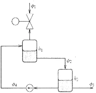
The quadruple-tank process is a simple connection of two double-tank processes, which are standard processes in many control laboratories. The setup is thus simple but still the process can illustrate interesting multivariable phenomena.

The process flow sheet is displayed in Figure 1. The target is to control the levels y 1 and y2 in the lower two tanks with two pumps. The process inputs are ul and u2 (input voltages to the pumps). The model used in the present virtual lab includes also the disturbance effect of flows in and out of the upper-level tanks.

v, v,

Figure 3.0: Schematic of the quadruple-tank process

Johansson (Johansson, 2000) described a laboratory quadruple-tank process which consists of four interconnected water tanks and two pumps as shown in Figure 1.0. The first principle mathematical model for this process is using mass balances and Bernoulli's law. The differential equations representing the mass balances in this quadruple-tank process are:

where hi is the liquid level in tank i;

ai is the outlet cross sectional area of tank i;

si(hi) is the cross-sectional area of tank i;

uj is the speed setting of pump j, with the corresponding gain kj;

'Y j is the portion of the flow that goes into the upper tank from pump j;

and di and d2 are flow disturbances from tank 3 and tank 4 respectively, with corresponding gains kdi and kd2.

The process manipulated inputs are u1 and u2 (speed settings to the pumps) and the measured outputs are y1 and y2 (voltages from level measurement devices).

The measured level signals are assumed to be proportional to the true level, i.e., y 1 =

km1hJ and Y2 = km2h2. The level sensors are calibrated so that km1 = km2 = I. (Astrom, I992)

This process exhibits interacting multivariable dynamics because each of the pumps affects both of the outputs. The linearized model of the quadruple-tank process has a multivariable zero, which can be located in either the left or the right half-plane by simply adjusting the throttle valves 'Y I and y2.

Johansson (Johansson, 2000) showed that the inverse response (non minimum phase) will occur when 0 < yi+ y2 <I and minimum phase for I< yi+ y2 :S 2. The valve settings will give then to the overall system entirely different behaviour from a multivariable control viewpoint. Unmeasured disturbances can be applied by pumping water out of the top tanks and into the lower reservoir. This exposes to disturbances rejection as well as reference tracking.

Values .I, .. \:'

.12 .. 1.;

(/. t .{lJ

fi:2 .iLl

!,,

l ern..: I

\cm2\

'''"''!

_!,m:\

j\':1'11/l

l'·''t/ . .:;~' I, ,_ '. I

Ill i( f

I Li i.~',.'j"

j _i -~·

Table

1.0:

Parameter value for quadruple

tank

system

( tpcrating Values

! /;;'

.h';

J

1^{{''1. • ;-,}

I I ; .11 1 I

'· ,.H 1"' ·.• 1'':_,, 1h.!:21

( -.. ! .-·,. 21

l'nits

\('m I

\Nn I II' I

' '\' lc!n- _:' .:::]

I' :12.1.12.7\

: !..".Ill

I :\.IJ(I, :l,l.ll_l ;.

J_:).:)~~.J.;r~l:·

(11.70.0.601

I'.

112 ii. t:l.Cii :U.l_q,

f J. u: .. :~. l-~~ j

(:L l L ~L2~.q

10.4:\.lt.:ll)

Table 2.0: Operating parameter for minimun (P-) and non-minimum (P+) phases

The linearized state-space equation at operating points are Xi= hi- h⁰i and ui = Vi- v⁰i

d.r

dt

l T,

u u

0

(I 1

---~

(I II

....

,. I-·, t :-1;1

. \ l

~ .\IT:

u

II

I ,

II

(.

·. k, 0

II I·

(I

li :: ) .1'

; ' ) , . d

where the time constants are

T ---

_{I - -} J... ·' .:::..:_;_ _n:

v

^{;I '}

0

___j_;_

.-\,T: .r

()

1/

Linearized transfer function matrix model for

both

^{minimum (P-)} and non-minimum (P+).

2.2 CURRENT PROCESS MODEL SIMULATION APPLICATION

2.2.1 Quadruple tank simulation

Most computer simulations of scientific phenomena can be described in terms of the model-control-view paradigm. This paradigm states that a simulation is composed of three parts:

1. The model, which describes the phenomenon under study in terms of

1. Variables, that hold the different possible states of n. The phenomenon

m. Relationships among these variables (corresponding to the laws that govern the phenomenon)

iv. Expressed by computer algorithms

2. The control, which defines certain actions that a user can perform on the simulation

3. The view, which shows a graphical representation of the different states that the phenomenon can have. This representation can be done in a realistic or schematic form

The tool provides extensive scaffolding for creating the model but still leaves full flexibility for the analysis. This is pedagogically important, since the process of analysing good control fundamentals consists, to a great extent, in to know the basic principles to build models. In order to describe a model, the simulation needs to be able to:

1. Identizy the set of variables that properly describe the system 2. Initialize, in a correct way, these variables

3. Describe how the value of these variables change in time

4. Establish how they affect each other when the user interacts with the system and modifies one or more of their values

5. Understanding control limitations due to interactions, model uncertainties, non-minimum phase behavior, and unpredictable time variations

6. Designing decentralized (often called "multiloop") controllers, and understanding their limitations

7. Implementing decouplers to reduce the effect of interactions, and understanding their limitations

8. Implementing a fully multivariable control system

9. Selecting the best control structure, based on the characteristics of the multivariable process

Past studies of (A. J. Krener, 1983) with 4-tank apparatuses implemented decentralized PI control, multivariable control, multivariable internal model control, and dynamic matrix control. The main educational focus was providing an apparatus with highly idealized and reproducible dynamics for use in illustrating multivariable interactions and multivariable transmission zeros as stated by Andersson (Andersson, 2002). In contrast, our main educational focus is to aid in understanding the advantages and disadvantages of the different control structures (e.g., decentralized, decoupling, multivariable) when applied to a multivariable process with interactions and dynamics ranging from highly ideal to highly non-ideal.

The main idea of this technique is to find some state transformation that make original system as a linear part, and nonlinear part depending only on measured states and inputs. The main drawback of this strategy is the difficulty to give necessary and sufficient conditions for existence of this transformation.

2.2.2 Developments in multivariable control simulation

Developing mathematical models of non-linear systems is a central topic in many disciplines of engineering. Models can be used for simulations, analysis of the system's behaviour, better understanding of the underlying mechanisms in the system, design of new processes and design of controllers. In a control system the plant displaying nonlinearities has to be described accurately in order to design an effective controller. In obtaining the mathematical model, the designer follows two methods.

The first one is to formulate the model from frrst principles using the laws governing the system. This is generally referred to as mathematical modelling.

The second approach requires the experimental data obtained by exciting the plant and measuring its response. This is called system identification and is preferred in the cases where the plant or process involves extremely complex physical phenomena or exhibits strong nonlinearities.

Obtaining a mathematical model for a complex system is complex and time consuming as it often requires some assumptions such as defining an operating point and doing linearization about that point and ignoring some system parameters.

In the present work three different models have been developed using three different soft computing techniques namely, ANN, Fuzzy and Neuro-fuzzy, for the Quadruple tank process. The rest of the paper is structured as follows: Section 2 describes the Quadruple Tank Process as stated by Rosenbrock (Rosenbrock, 1973).

2.2.3 Easy-Java simulations fundamentals

As stated by (Esquembre, 2002), Easy Java Simulations, Ejs for short, is a software tool that helps create dynamic, interactive scientific simulations in Java language. The tool is targeted for basic programming skills and is therefore very much suited to the pedagogical situation one finds in most university classrooms. Within Ejs, simulations are created by specifying a model for the simulated system and by building a view that continuously visualizes the state of this model and that readily responds to user interaction.

CHAPTER 3: METHODOLOGY/PROJECT OF WORK

3.1 METHODOLOGY

3.1.1 RESEARCH METHODOLOGY

Proce-;;, model deriYation

Simulation illltial kst

Suunlate & te-;t of se·1eral kinds of decepllon

Generation of Input-Output Data

\"ahdation ... -

J

---...

/ / \"ahd" ,

,. >---l

···-...

Data analvm

E.ud

^-,..,_ _'

/

Figure 5.0: Research method flowchart

3.2 PROJECT ACTIVITIES

3.2.1 Process model derivation

The model theoretical design of quadruple tank model is referred as the main reference throughout the whole process of developing the dynamic simulation. All parameters are recognized, derived and all variables are defined.

Constant variables:

i. Al, A2, A3 and A4 are the cross-section area of each tank

11. ai is the cross-section area of an outlet of the tank iii. g is the gravitational constant, 981 cm/s²

Manipulated parameters or input:

i. Voltage of the pumps

11. Ratio of the flows

Output parameters:

i. Speed settings to the pumps ii. Tank level

Process model:

dh ~ zeros(4,1);

dh(l) ~ -al/Al*sqrt(2*g*h(l)) gl_nrnp*kl_nrnp/Al*ul;

dh(2) ~ -a2/A2*sqrt(2*g*h(2)) g2_nrnp*k2_nrnp/A2*u2;

dh(3) -a3/A3*sqrt(2*g*h(3)) dh(4) ~ -a4/A4*sqrt(2*g*h(4))

+ a3/Al*sqrt(2*g*h(3)) + + a4/A2*sqrt(2*g*h(4)) + + (l-g2 nmp)*k2 nmp/A3*u2;

+ (1-gl-nrnp)*kl-nrnp/A4*ul;

- ^-

3.2.2 Software set up

Apply the tools of software which are MATLAB® and Simulink. Coding and mathematical expression and functions are prepared using the tools. Whole system is then developed in order to run the whole dynamic simulation of the quadruple tank system.

The algorithms used in the ODE solvers vary according to order of accuracy and the type of systems (stiff or non-stiff) they are designed to solve. The solvers of the ODE suite can solve problems of the form lv[(t, y\y' = f(t. Yl, with time- and state-dependent mass matrix

M.

Solver Problem Order of When to Use

Type Accuracy

ode45 Nonstiff Medium Most of the time. This should be the first solver you try.

ode23 Nonstiff Low For problems with crude error tolerances or for solving moderately stiff problems.

odell3 Nonstiff Low to high For problems with stringent error tolerances or for solving computationally intensive problems.

ode15s Stiff Low to If ode45 is slow because the problem is medium stiff.

ode23s Stiff Low If using crude error tolerances to solve stiff systems and the mass matrix is constant.

ode23t Moderately Low For moderately stiff problems if you need a

Stiff solution without numerical damping.

ode23tb Stiff Low If using crude error tolerances to solve stiff systems.

Table 3.0: ODE's Function in Matlab

3.2.3 Simulation initial test

This method is to calibrate the system developed using MA TLAB® and Simulink. This is to prepare a good generation of data during the simulation.

Sample ofMatlab coding for Run 1

function dh

-, ~-· - ,-c ~~, c: ~: 3 ·~·, A1~28;

A2=32;

A3=28;

A4~32;

al~0.071;

a2~0.057;

a3~0. 071;

a4=0.057;

height(t,h)

:_, l_ ,f; J ,_-:·

kl_nmp 0.5;

k2_nmp 0.5;

gl_nmp 0. 70;

g2_nmp~ 0.30;

ul~0.5;

u2=0.5;

dh ^~ zeros(4,1);

dh(l) = -al/Al*sqrt(2*g*h(l)) + a3/Al*sqrt(2•g*h(3)) ^~ gl_nmp*kl_nmp/Al*ul;

dh(2) = -a2/A2*sqrt(2*g*h(2)) + a4/A2*sqrt(2*g*h(4)) + g2_nmp*k2_nmp/A2*u2;

dh(3) -a3/A3*sqrt(2*g*h(3)) + (l-g2 nmp)*k2_nmp/A3*u2;

dh(4) = -a4/A4*sqrt(2*g*h(4)) + (l-gl=nmp)*kl_nmp/A4*ul;

The function is called and the graph is plotted for data display.

[T, H] = ode45 (@height, [0 120]. [0 0 0 OJ);

plot(T,H(:,l), '--',T,H(:,2), '*',T,H(:,3),' ',T,H(:,4),'.');

3.2.4 Generation oflnput-Output Data

The data generated to train the network should contain all the relevant information about the dynamics of the Quadruple tank process. The input was given to the conventional model of the quadruple tank process, and from the conventional model, the input and output were sampled for each sampling instant and the required sampled data are obtained to train the network.

The quadruple tank system is divided with several conditions in order to define dynamic behaviour in the process by simulation.

1. Steady states

The first simulation is to take measures in one or several steady states of the process (with several the mean value of the results is taken), knowing that if a dynamical system is in steady state, the rate of change of the state (h) is null.

2. Valve constants

dh ~o dt

Y1 and y2 is derived. For that, all the output holes of the tanks must be covered, so that the first addends of all the expressions disappear, and consequently, second addends of the first and second equations have to be also removed. The simulation for valve constants is run.

If that input is constant, a derivative can be expressed in non-inf"mitesirnal time periods.

{1\ .::.:r

---'-- !::i - · · ·

dt ,;j.

'\ii -k .::::...:..:::::-'-11

::.J AI

\i' ~

~;;:;:~·-·--~~

.;;,f .-L. .

_, .{

The parameters k~, u~, k2, u2 are constant, as A~, A2, A3.

AJ,

^Moreover,

the simulation's time doesn't matter, because it can be added to the constant member

kc,

considering A1 =A2 = A3 = ~-

3. Water tanks hole areas and pump constants

In this section, the values of the following not directly measurable parameters k~, k2, ab a2, a3, 14 are derived, knowing A~, A2, A3. ^~ those are easily measurable.

4. Parameters values and final model

Values ai of holes areas and k of the pumps are obtained just substituting values of bi in the first simulation to take ci and undoing the variable changes of both kinds of variables. These last parameters are:

A1 =A2 = A3 = ~ = 15.21 cm2 a1 = 0.2143 cm2

a2 = 0.173 cm2 a3=0.2102cm2 14= 0.1793 cm2 k1 = 4.0356 cm3

Ns k2= 3.9375 cm3Ns

Therefore, the final model with minimum phase configuration is the following:

-,,t-1 0 0 '_Y;J ^~n o

0 -C.5C3S

(I

~I

I ' - "'

o-_ h~ : 0 ^-

'li'.

_h,~ ^{' '}

This model of simulation is linearized to design the linear controllers chosen in this thesis, and the derivation of the model is repeated for the non-minimum phase process, with the same parameters.

3.2.5 Validation

The final step in developing the model is validation of the generated results of the simulation. Validation is performed by evaluating the simulation performance using trained or experimental data and test data. The input and target were presented.

If the data is not valid within the range of validation, the method is re-looping start from the simulation initial test. If the data is valid, the data is analysed.

3.2.6 Data analysis

Data analysis is performed by comparing the expected results and data referred to the previous valid data of previous experiment of quadruple tank system. Several considerations are important;

1. The effect of time-varying dynamics should be considered when designing contro I systems

2. The sign of the steady-state gain should always be considered when designing control systems for multivariable processes

3. The cause of unexpected dynamic behaviour in control loops is often more subtle than what is first assumed

4. Under some conditions, full decoupling can lead to significantly worse performance than partial decoupling

5. Decoupling control can do more harm than good

6. Hysteresis effects should be considered when troubleshooting control problems

CHAPTER 4: RESULTS AND DISCUSSION

4.1 RESULTS

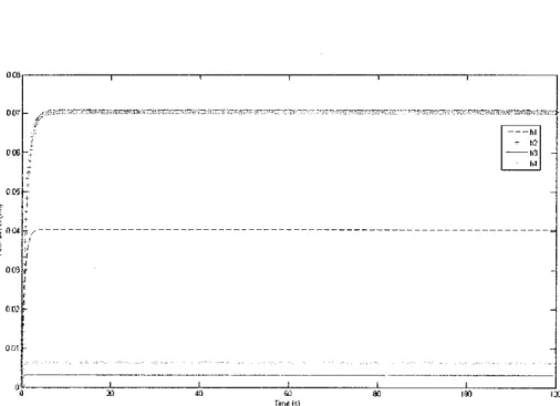
4.1.1 Steady states

Take measures in one or several steady states of the process (with several the mean value of the results is taken), knowing that if a dynamical system is in steady state, the rate of change of the state (h) is null.

function dh = height(t,h) A1=15.21;

A2=15.21;

A3=15.21;

A4=15.21;

a1=0.2143;

a2=0.1773;

a3=0.2102;

a4=0.1793;

g=981;

kl_rnnp 4.0356;

k2_rnnp 3.9375;

gl rnnp = 0.69;

g2_rnnp= 0.74;

u1=0.5;

u2=0.5;

dh = zeros(4,1);

dh(l) = -al/Al*sqrt(2*g*h(l)) + a3/Al*sqrt(2*g*h(3))

*

gl rnnp*kl rnnp/Al*ul;

cth(2) = -a2/A2*sqrt(2*g*h(2)) + a4/A2*sqrt(2*g*h(4}) + g2 nmp*k2 nmp/A2*u2;

cth(3) -a3/A3*sqrt(2*g*h(3)) + (1-g2_nmp)*k2_rnnp/A3*~fi dh(4) = -a4/A4*sqrt(2*g*h(4)) + (1-gl_nmp)*kl_nmp/A4*ul;

[T,H] = ode45(@height, [0 120], [0 0 0 0]);

plot(T,H(:,l), '--',T,H(:,2), '*',T,H(:,3), ¹ ',T,H(:,4), I . ' ) ;

ore,---,---,---,---,---,---,

our

000

ON'

K ]~~;r---· ---

~ ;/

~ _,

'

OOl,

0(.1;>

ODt J

'

""

Figure 4.0: Simulation results for steady state condition

4.1.2 Valve constant

Outputs of closed loop ~Nith P! cont~·o11el~ and mmimurn phase zero model

2.---~---.---.----~--~---.----.---.---,

0

-2

g -4-

!:>

:E ""

~· ·6

-8

-10 _)

. 12 '---"::---::-'-:---:-"-::---'-,---,:-:L--c-'-c---,-Jc---:-"-::---::-'

0 100 200 300 400 500 GOO /00 800 900

T1rne (s)

Control actions Closed loop with PI controllers and mlnwnurn pha-::.e zero model

15 .--~-~--.--.--.--.--~--.---,

: i '

0.5 I

o

I r<·:--- ---

f·:

^_Ill

-1.5 -2

I

-2: j

· j o""----=1~o"o---"'<oo':;_,---:3~0C::::_,----:40'c,o,---;5~o"'o--::G:Ooo:::---=7='o"o----:-::8:000:::---:c:::'_,o-o

Twne (s)

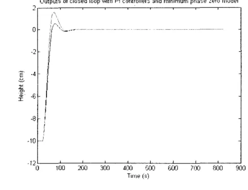
Figure 5.0: Results of minimum phase zero configurations

O!Jtputs of dosed loop ..,...rith PI controllers .;md non-minimum ph:..se z.em mo(Jel 2~---.-~.---,---~--~--~---.---,

0

-2

,.· ;>--,=--- ---

i/ :'/

.ti il

~- -4

:.=.

)

:/

>-:

'"

c 0

~ e

§

'-"

_II

I

8

I

i

-10

-12 ·--.-o,to .. _-,-_"--"~-=:l.,-.~-,-,-. '"-~-1--,.

0 100 D D 0 ~ @ ~ 0 ~

Time (s)

Control actiom;. Closed loop with PI controller;; .:md n.:•rHiilriln··,iJrn t•iril§>?" zpro model

05 ---c~-r-'--~--

0

(>''2=

-0.5

//

-1

I/

-1.5

r

-2

-2.5

_,

3.c ';--;;~-;;;~-;;;~---;;~~;;c--;c'!;,----d~--dc:---;::!

-~ 100 D D 0 0 ~ ~ 0 D

Tmw {s}

Figure 6.0: Results of non-minimum phase zero configurations

The responses have overshoot because of the influence of upper tanks, but it is not really high, even knowing that the step applied is wide, and applied from a long distance point from the equilibrium one. The response is better in non-minimum phase zero model because of the decoupling applied to obtain a stable system. The applied voltages are not much more than IV over the linear OV, no more than 5V adding the linearization values. Knowing that the saturation level is 12.5V, it can be said that there will be no problems with this saturation. All the states are observed during the simulation, and upper tanks don't have problems of overflow, as the lower ones. With these conclusions, and taking into account possible differences between process and model, the following step is to test the controllers in the real process.

4.1.3 Water tanks bole areas and pump constants

§ 6

-10

-l:20':----:5C;;O----,,C:::00;----;-;15::;-0 --~:!C~J

T1me (>.)

Estimated states

2~---~---~

-10

. "':----:";c----:=---:-;::;---~

o -:o ^{100 150 200}

T1me (s)

Control act1ons

2 3.5

c ~ 3 ^I

~

~ 2.5 !

~ w

--2 2 I :l, ~ t5 ^0'!:.·.·

"fj 0 M

'2 c

0 0.5

u

u !

L

-

~

Q c-._~,.r-~L.Fl.,__,-,__F-'r,_~--J":.:~: -~-=..F~:::"--cfj"'-._r::l ... J"'...::'J"'~ .. ~ ~---~~

-0.5 ':----:",----:':---::'::---:':---:-!'-:--~::---c-'-:-'----,~'--:-!'':---:"

o 20 40 Gil ao 100 120 140 160 tao 200

T1me (s)

Figure 7.0: Simulation results. Process model with minimum phase zero

The response of states 1 and 2 is better than states 3 and 4, without overshoot and relatively quicker (taking into account the difference of distance to the equilibrium point). The variation of control actions is smooth too, not osciliating around the control actions in equilibrium point. Therefore, the response in simulation is what could be expected according to the design. In addition, ahnost the same result is obtained with the model process with non-minimum zero.

4.1.4 Deviation

To determinate the deviation, a simple simulation is done. Constant control actions of 1 OV are introduced. Heights data have to be captured during a relatively long time, to obtain correct mean values and therefore valid deviations. In this case, 235 samples are obtained:

E~

·~-·

..:: f!

'(ii =

::t:

18~--~--·---~--~--~--~--~~~~~~

--Hei1Jht1

1 G - ---- -Height 2

14

r\/t{'t'llvt'i!V .. hf~WV.''··'V-V·i\ll/i~\\.~t',_}\lfif''1/Y\.f~A\/'i'ILN''i~-.,i-.~"~'\·i·~-'d.)-''·'·'~,~.i-·

12

10 -

8

6

4

~~--~~--~--~~--~~~~----L---~----~·~---L--~

k 0 50 1 00 150 200 250 300 350 400 450 500

Tu-ne (:;)

Figure 8.0: Deviation of level Tank 1 and Tank 2 for 470 seconds

4.1.5 Parameters values and final model

Some steps are introduced around the equilibrium point to test the behavior, changing dynamically the linearization point, and therefore changing the model too.

Seeing some parts of the simulation, made with minimum zero process:

'E

Estirnated st-ates ;;.fith real proO?$S. Gitli•p fit11Yi W to 8cm

12~~-~~~~-~~-,====:::c::=::::;l

X= 102 'I= 10.263 10

8

~·1

X= .,-,~)

~~ ,;=8~0:3t

--Heigh11 Heoghl 2

-~---- Heoghl 3 Heoghl A

~-~--~.<::-~~~--·

-~ .c ⁶

·;;; ~

I

A

2

0 .I

80 90 100 110 UO 130 140 150 1Eo0 170 180

Tome (oo)

Pump contto! acllons. Step f10rn 10 to Bern

6~~~--~~~--~~r=~=c~

-~-Voltage 1

58 ---- --· \/oltage 2

56 5.4

< _'L

L..J~~

'

'""~

i

I

A8 At'

n

^{1._ ~,n_.-,_,}

-I rn

i

I

AA I _.I

l

_--; ^{1 .. 1}

~

90 100 110 120 130 140 150 160 170 180

Time (s)

Figure 9.0: Simulation behavior with a step from 10 to Scm. Minimum zero configuration

As it can be observed, the dynamical response is adequate with design criteria.

Changes in the heights are quick (settling time of 20 seconds), with good exactitude for the 2 first states, and a good noise filtering. In addition, first samples after the change of reference have a remarkable peak. This happens because of the change of model.

Regarding to the control actions, they have a bigger overshoot, but just to bring the state of the system as fast as possible to the equilibrium point. This happens because of bigger weightings of heights I and 2 than the ones of both voltages. The same result can be seen in another experiment, this time with non-minimum phase zero configuration:

7

"' 6.5 0

m c

0

13 _~ h - 2

"

⁰

u 65

5

Estimated -:>t<-1tes with re<~l process_ Step from 8 tc• 11 em

12,----r----~--~---~----~---.

11

tO 9

5 4 3

Twne ls)

Pump control act1ons. Step from 8 to \!ern

4 5 '-::---::-L:----:-::c---:"::---::-'::----:::'-::---::-'-:---::'

220 240 260 280 300 320 340 360

Tm)e (';)

Figure 10.0: Simulation behavior with a step from 10 to Scm. Non-minimum zero configurations

4.1.6 Validation

The dynamics are accurate, but what can be noted is that there's a delay provoked by the length of the tubes. There are 3 to 4 samples until the effect of an input change is noted in an output.

Validation. h~eal vs Simulated ouiput'B

16 , - - - . - - - , c - - - , - - - , - - - - . - - - - r - - - , 14

12

!' . .;~, .~t,

-·~(~---···

.E. 10 ,-_-::·1

~~

E 8

""

"Q:j I

5

4 ^.

---Simulated height 1 2 ^.

--····- -Simulated height 2 ----Real height 1

Real height 2

0 0 100 200 300 400 500 1300 700

Time (s)

Figure 11.0: Validation

The gain model is correct around water levels of !Ocm. With measures of between 12 and 14cm, the gain of the real system is higher. This happens because of the time variable behavior of the pumps and sensors. Some experiments with a separation of days between them have different results. In general, it can be said that the model is valid around lOcm, which will be the point used for most of the simulation. The dynamics are accurate, but what can be noted is that there's a delay provoked by the length of the tubes. There are 3-4 samples until the effect of an input change is noted in an output. The gain simulation is correct around water levels of

!Ocm. With measures of between 12 and l4cm, the gain of the real system is higher.

The different percentage is 14.02% based on the average for every heights.l4.02% is lesser then 15%, which is the targeted percentage difference. The data in the simulation is validated.

CHAPTER 5: CONCLUSION AND RECOMMENDATIONS

5.1 CONCLUSION

The Quadruple-Tank Process has been presented. It is a simulation process that was designed in order to illustrate various concepts in multivariable control. It has been observed that in each design technique, non-minimum phase is quite difficult to control. Multivariable system with unstable transmission zeros usually come across with internal instability problems. The sign of the steady-state gain should always be considered when designing control systems for multivariable processes. This level of understanding is needed to select the proper design of quadruple tank system and to determine whether a particular control problem can be addressed by better controller tuning, by a different control structure, by changing the process design, or by changing the operating conditions.

Dynamic simulation of multivariable process for quadruple tank system is developed using MATLAB® to study the dynamic simulation of quadruple tank system. The complexity of the dynamics of the system can be represented by the graph and data deviation of the height of each tanks controlled by the vohage of each pumps.

The state of variables which are height and voltage of the pump are validated by the real process of quadruple tank system. The feasibility design of quadruple tank system can be determined by this simulation.

5.2 RECOMMENDATIONS

The project is generally at the stage of process model derivation, input and output generation and validation to get more understanding about the quadruple tank system. The coding of the MATLAB® would be the time consuming but the project should be managed to continue to the next steps till the end by the scheduled project of work. Further research and reference is relevance in order to make sure the results of the dynamic simulation is valid and the objective of this project can be achieved.

REFFERENCES

A. J. Krener and A. lsidori, Linearisation by output injection and nonlinear observers, Syst. And Cont. Lett., vol. 3. 1983, pp 47-52.

Andersson, M.; Glad, T.; Norrl6f, M.; Gunnarsson, S.: (2002). A simulation and animation tool for studying multivariable control. 15th World Congress of!FAC, Barcelona 21-26 July.

Astr6m, K. J.; Lundh, M.: (1992) Lund control program combines theory with hands-on experience. IEEE Control Systems Magazine, vol 12, n° 3, pp. 22-30.

Esquembre, E.: (2002). Easy Java Simulations 3.1, http://fem.um.es/Ejs

K. H. Johansson, The Quadruple- Tank Process: A Multivariable Laboratory Process with an Adjustable Zero , IEEE Transactions on Control Sytems Technology,

8(3), (2000), 456-465.

Qamar Saeed, Vali Uddin and Reza Katebi, Multivar iable Pr edictive PID Control for Quadruple Tank, World Academy of Science, Engineering and Technology 67,2010.

R.Suja Mani Malar and T.Thyagarajan, Modeling of Quadruple Tank System Using Soft Computing Techniques , European Journal of Scientific Research, 2009.

Rosenbrock, H. H. (1973). The zeros of a system. International Journal of Control18, 297-299.

Salt, J.; Albertos, P.; Dormido, S.; Cuenca, A.: (2003). An interactive simulation tool for the study of multirate sampled data system . 15th IFAC Symposium on Advances in Control

APPENDICES

function dh height(t,h)

- ':;: ^~~-::' ;:_,-, '- ' ,-:. t A1~28;

A2~32;

A3~28;

A4~32;

al~O. 071;

a2~0.057;

a3~0.071;

a4~0.057;

g~981;

kl_nmp 0. 5;

k2_nmp 0.5;

gl nmp ^~ 0.70;

g2_nmp~ 0.30;

, " ' - -ir-;r• -,/'!

-'':_.,-

ul~0.5;

u2~0.5;

dh ~ zeros(4,1);

APPENDIX 1-1

dh(l) ~ -al/Al*sqrt(2*g*h(l)) + a3/Al*sqrt(2*g*h(3))

*

gl_nmp*kl_nmp/Al*ul;

dh(2) ~ -a2/A2*sqrt(2*g*h(2)) + a4/A2*sqrt(2*g*h(4)) + g2_nmp*k2_nmp/A2*u2;

dh(3) -a3/A3*sqrt(2*g*h(3)) + (1-g2 nmp)*k2 nmp/A3~uz;

dh(4) ~ -a4/A4*sqrt(2*g*h(4)) + (l-gl=nmp)*kl=nmp/A4*ul;

[T,H] ~ ode45 (@height, [0 120], [0 0 0 0]);

plot(T,H(:,l}, '--',T,H(:,2), '*',T,H{:,3},' ',T,H(:,4),'. ');

package QuadTankPack

model PRBS1

Modelica.Blocks.Interfaces.Real00tpu·~ y;

parameter Integer N ~ 10;

parameter Real ts[N] ^~ 24.3, 36.3, 39.3, 42.3,

0. ^f ~~.;J,

54.3, 57.3);

APPENDIX 1-2

9.3, 15.3,

parameter Real ys[N] { 5., 6., 5., 6., 5., 6 , 1 5 • r 6 • 1 5 , f 6 ,· } ;

equation

y ^~ noEvent (if time ^<~ ts [2] th~ri j!J l ^I l ^(~lse

i f time ^<~ ts I ^{3] thicJJ.'! y~~ [ 2] oo:-;L3§}

if time ^<~ ts ^{[ 4]} then ys ^[3] el.se i f time ^<~ ts ^{[5] thsn} ys [ 4] ~~1§§

if time ^<~ ts [ 6] th~!ll ys ^[5j t~.l-f>i@

i f time ^<~ ts

[II

^{th(fi1 ys [61}

if time ^<~ ts [ 81 ^ttl8:ft ys [ 7 J if time ^<~ ts [9! ^tiv~Jl vs lsI

if time ^<~ ts [10] then V"' ^•0 [ ~} j ~.t.f.<'.': ys [ 10] ) ;

end PRBS1;

model PRBS2

Modelica. Blocks. Interfaces. RealOutpt~ ( y J

parameter Integer N = 11;

parameter Real ts[N] ~ I 0.

24.3, 27.3, 39.3, 42.3, 48.3, 51.3, 57.3);

0. 3, 9.3, 21.3,

parameter Real ys[N]

5., 6., 5., 6., 5.};

{5., 6., B"~' 6., s., 6.,

equation

y ^~ noEvent(if time ^<~ ts [2] then ys[l]

if time if time if time if time i f time if time if time if time if time end PRBS2;

model TestPRBS PRBSl prbsl;

PRBS2 prbs2;

Real x;

equation der(x) ~ 1;

end TestPRBS;

<~ ts [3] then

<~ ts [ 4] then

<~ ts [ c•J l~hG1fl

<~ ts [ 6] then

<~ ts['ij ti"-Jen

<~ tsf8] ^th~;;n

<~ ts [ 9] t.lv~n

<~ ts [llJl ^eh~:~H,

<~ ts [11] then

model Sim_QuadTank QuadTank qt;

input Real ul input Real u2 initial equation

der (qt.xl) 0;

der (qt.x2) 0;

qt.x3 ~ 0.024;

qt.ul;

qt.u2;

ys [2] else

ysfJ"] §@

j'f1[ 4] else

ys[ 6188

ys [ 6]

ys [7j ol&©

ys[8i ~~ J-.~3

ys l ';J

ys [ 10] else

APPENDIX 1-3

else

ys [11] I ^;

qt.x4 ~ 0.023;

end Sirn QuadTank;

model QuadTank

II Process parameters

parameter Modelica.Siunits.Area A1~4.9e-4, A2~4.9e-4, A3~4.9e-4, A4~4.9e-4;

parameter Modelica.Siunits.Area a1~0.03e-4, a2~0. 03e-4, ^a3~0. 03e-4, ^a4~0. 03e-4;

APPENDIX 1-4

parameter Modelica.Siunits.Acceleration g~9.81;

parameter Real kl_ nrnp (uni t="m3{\ I s/ll")

k2 nmp(unit="m"3/s/V") = 0.56e-6;

parameter Real gl_nmp~0.30, g2_nmp~0.30;

II Initial tank levels

parameter Modelica. S Iuni t~:. 1oJf~nqGh )~l, 0 0.04102638;

parameter Modelica. Siuni t.':"l. IJ§f1(f'Gh ~'~~ 0 0.06607553;

parameter Modelica.Siunits.L~figth x3 0 0.00393984;

par·arneter Modelica. Siuni ts. 1j~Hi.gth :J{4 0 0.00556818;

II Tank levels

Modelica.Siunits.Length

x1 (start~x1 O,min~0.0001/''·,max~0.20'•/j 1 Modelica. S Iuni ts .l&mgth

x2 (start~x2 O,min~0.0001I'•,mcL~ •0.20*/);

Modelica.Siunits.Length

x3(start~x3 O,min~0.0001/'·,max~0.20""111

Modelica.Siunits.Length

x4 (start~x4 O,min~0.0001/',mc1x~0.2(1'11 f

APPENDIX 1-5

II Inputs

input Modelica.Siunit~;.Voltagc U}J input Modelica.SIU11i-ts.Voltay~ J2i

equation

der(xl) -aliAl*sqrt(2*g*xl) + al/Al*sqrt(2*g*x3) +

gl_ nmp* kl nmpiAl *ul;

der(x2) -a2IA2"'sqrt (2*g*x2) + a4IA2*sqrt (2*g''x4) +

g2_nmp"'k2 nmp/A2''u2;

der(x3) - -a3/A3*sqrt(2*g*x3) + (l- g2 nmp)*k2_nrnpiA3*u2;

der(x4)- -a4IA4*sqrl;(2*g'ou1) (I~

gl nmp)*kl_nrnpiA4*ul;

end QuadTank;

model QuadTankinit extends QuadTank;

initial equation der(xl) 0;

der (x2) 0;

der(x3) 0;

der(x4) 0;

end QuadTankinit;

optimization QuadTank_Opt (objective "- CoB[ (final Time), startTime 0,

final Time 50 I

APPENDIX 1-6

extends

QuadTank(ul(initialGuess=ul r),u2(initia1Guess=u2 r), xl(initialGuess=xl O,fixed=true), x2(initialGuess=x2 O,fixed=true),

x3(initia1Guess=x3 O,fixed=true), x4(initialGuess=x4 O,fixed=true) );

II Reference values

parameter Modelica.Siunits.Length x1 r 0. 06410371;

parameter Modelica.Siunits.Length x2 r 0.10324302;

parameter Modelica.Siunits.Length x3 r 0.006156;

parameter Modelica.Siunits.Length x4 r 0.00870028;

parameter Modelica.Siunits.Voltage ul r 2. 5;

parameter Modelica.Siunits.Voltage u2 r 2.5;

Real cost(start=O,fixRd³ trlle);

equation

derlcost) 40000* I ( x l r - xJ) j ii~ !~

40000* I I ,~::j I '·2 + 40000* I lx3 r - ^!: ·q) A2 + 40000*1(x4 r - ~n))·~ +

((ul r - u:i_j}'':? ¹

end QuadTank Opt;

APPENDIX 1-7

optimization QuadTank Static(objective~( ~1 rneas-x1)~2 + (x2_meas-x2)A2 +

(x3_meas-x3)"2 + (x4_meas-x4)'2, static~true)

extends QuadTank(al(free~true),a2(free~true) );

parameter Real xl me as 010.01;

parameter Real x2 me as :<2 0··0.01;

parameter Real x3 me as s3 _.. 0-0.0J.;

parameter Real x4 me as ^;<4j 01-0.01;

initial equation der (xl) 0;

der(x2) O· _' der (x3) o· _'

der (x4) 0;

end QuadTank_Static;

optimization QuadTank ParEst (objective~sum((yl_meas[i]

- qt.xl(t_meas[i]))A2 +

(y2_meas[i]

- qt.x2(t_meas[i]))A2 f o r i in l:N_meas),

startTime~O,finalTime~60)

II Initial tank levels

parameter Modelica.Siunits.Length ~:1 0 0.06255;

parameter Modelica.Siunits.Length x2 0 ^0.06045;

parameter Modelica.Siunits.Length x3 0 parameter Modelica.Siunits.Length x4 0

QuadTank qt(xl(fixed~true),xl O~xl 0,

x2(fixed~true),x2 o~x2 0,

x3(fixed~true),x3 o~x3 0,

x4(fixed~true),x1 01

al(free=true,initialGuess 4,nominal=0.03e-4,min=O,max=O.le-4),

a2{free=true,initialGuess

4,nominal~0.03e-4,min~O,rnax~O.le-4));

parameter Integer N_meas = 61;

APPENDIX 1-8

0.02395;

0.02325;

0.03e-

0.03e-

parameter Real t_meas[N_meas] 0:60.0/(N meas- 1) ; 60;

parameter Real yl_rneas[N_rneas] ones(N_meas);

parameter Real y2_meas[N_meas] ones(N_meas);

PRBSl prbsl;

PRBS2 prbs2;

equation

connect(prbsl.y,qt.ul);

connect(prbs2.y,qt.u2);

end QuadTank_ParEst;

optimization QuadTank_ParEst2 (objective~sum((yl_meas[i]

- qt.xl(t_rneas[i]))A2 +

(y2_meas[i]

- qt.x2(t_meas[i]) )A2 +

(y3_meas[i]

- qt.x3(t_meas[i]) )A2 +

(y4_meas[i]

- qt.x4(t_meas[i]))'2 fori in l:N_rneas),

startTime~O,finalTime~60)

II Initial tank levels

pararneter·Modelica.S