1
CHAPTER 1 INTRODUCTION
1.1 Background of Study
Existing EOR methods in Oil and Gas Industry
During the past forty years, a variety of enhanced oil recovery (EOR) methods have been developed and applied mostly in depleted oil reservoir [1] in order to improve the efficiency of oil recovery compared with primary (pressure depletion) and secondary (water flooding) method. Using EOR, we can increase about 30% to 60% of the reservoir’s original oil compared with 20% to 40% using the primary and secondary recovery.
EOR generally involves four methods, which are listed below [1];
1. Thermal recovery which is about the injection of hot steam to the second drilled hole. The steam will be used to heat the crude oil either during its flow upward in the drill head or in the pool, which would allow it to flow more easily toward the drill head. The introduction of heat such as the injection of steam is to lower the viscosity or thin the heavy viscous oil and improve its ability to flow through the reservoir.
2
Figure 1: Thermal Recovery [2]
2. Chemical injection is applied by injecting the chemical substances like polymer into the reservoir to reduce the oil viscosity and increase the water viscosity.
Figure 2: Chemical Injection [3]
3
3. Gas injection method is using the carbon dioxide gas, C02 or other natural gases like nitrogen where those gases are injected to the reservoir. The expansion of the C02 gas into the reservoir cause the oil is breaking up into droplet and easier to be pumped. Some of the natural gases used for injection purpose dissolve in the oil so as to lower the viscosity of the oil thus aiding in its enhanced extraction.
Figure 3: Gas Injection [2]
4. Seismic approach where by using this method, the oil trapped in the rock matrices is being ‘vibrated’ by the sound wave and then pumped up.
Figure 4: Seismic Approach [4]
4
Alternatively now, researcher found that EM waves have a big potential to be used as one of the EOR methods [5]. The characteristic of the EM waves that can penetrate deep through the reservoir itself be the main asset of why EM waves got the potential to be used inside the reservoir. Nowadays people use the EM waves to detect the hydrocarbon reservoir [6]. Hydrocarbon plays a very important role in dealing with the geometrical survey of the sub-surface structure.
This alternative method is used for the same objective, to maximize the crude oil production by at least with about 10% increment.
1.2 Problem Statement
Most wells produce complex, fractal drainage patterns that cause the oil to trap within the rocks. Low temperature and high pressure below 1000m cause the flow of fluid (oil) remain a challenge and this make the industrial to face a problem in improving the mobility of the heavy oil.
1.3 Objective and Scope of Study
1. To design and construct a transmitter that can transmit powerful EM waves to a core sample.
2. To evaluate the effect of electromagnetic waves diffusion to the crude oil mobility.
3. To calculate the oil recovery using EM method.
5
CHAPTER 2
LITERATURE REVIEW
2.1 Electromagnetic Waves
Maxwell equation stated that the magnetic field produced (B) is proportionally related to the current and the type of material used. The bigger current flow inside a conductor, and the higher the permeability of the material used, the bigger B field is produced [7].
Magnetic field (B) and the electric field (E) is propagating together perpendicularly with the same amplitude where the reduction in B field intensity will cause the same amount of reduction in E field as well [7].
Figure 5 shows how the E-field and B-field propagating perpendicularly in a medium and Figure 6 shows that the magnitude of E-field is proportional to the magnitude of B-field.
Figure 5: Electromagnetic Waves propagation [8]
6 Based on Maxwell equation [7],
r B I
π μ 2
= 0 where;
B = Magnetic field,
µ0 = Magnetic Permeability I = Current (A)
r= Distance
Overview by Peter Signell from Michigan State University, it is possible for E-field and B-field to propagate as waves in the empty space or we said as vacuum [9]. Electric and magnetic wave’s field may exist in space without a material medium being present and if they vary in space and time in the appropriate way, the spatial variation will propagate as a wave, transporting energy. This module deals with the propagation of energy through a vacuum via electromagnetic disturbances whose space and time variation satisfy the conditions for wave propagation.
Figure 6: B field and E field propagation [10]
7 2.2 EM Transmitter and EM Detector
EM transmitter is defined as a radial waveguide that generates the EM wave while receiver is a radial waveguide that detects the EM wave [10]. Usually an EM transmitter uses turns of coil to generate the electromagnetic wave that is at a single frequency. When we apply a high frequency source of alternating voltage input to the coils/winding of the transmitter, a magnetizing current is developed in the winding itself. This magnetizing current then will generate an alternating flux in the magnetizable core that links the winding in order to develop an alternating polarity output voltage [11].
The amount of current induced depends on the electrical conductivity of the material itself [12]. Commonly we use copper as the transmitter since it is a highly electrically conductive material.
The currents induced in the transmitter then will generate a secondary EM field that can be detected using a receiver [12].
Commonly magnetic material like ferrite is used to construct the receiver. Magnetic material basically has the ability to gather or to concentrate the magnetic fields which then govern to the second induced currents [8].
The depth of penetration of the induced current can be calculated by using the skin depth equation. The smaller the skin depth will cause more induced current to concentrate at the skin of the magnetic material which will generate heat due to the eddy current.
Overviewed by Alex Becker, Ki Ha Lee and Lou Reginato form University of Califonia on downhole EM transmitter using a 100m deep well at Richmond field station [13], EM transmitter was tested its performance toward the barehole to the surface configuration with a receiver and the result shown that EM transmitter specifically suited for subsurface use where the transmitted EM waves could be detected by the receiver. The designed EM transmitter was based on a long solenoid with a non-dissipative magnetic core. This finding shows that EM transmitter could be potentially applied to the reservoir which has fractional drainage pattern [13].
8 2.3 Radiation and Antennas
Shape and size of a transmitter determine how effective it is in extracting energy from the radio wave. Usually an antenna is designed so that it can radiate or receive electromagnetic energy with directional and polarization properties suitable for the intended purpose or application [7]. In order to design a transmitter, it is important to know the resistance of the antenna itself. The radiation and resistance properties of an antenna are governed by its shape and size and the material of which it is made.
The resistance and conductivity of an antenna has the relationship as follows [14]; A
R
ρ
l= And
ρ
=α
1 Where; R= Resistanceρ
= Resistivity α = Conductivity l= LengthA= Area
Radiation sources are classified into two groups; currents and aperture fields [7].The dipole and loop antenna are examples of current sources while a horn antenna is one of the aperture source examples [7]. For current radiation source, the time- varying currents flowing in the conducting wires give rise to the radiated electromagnetic field [7]. In aperture source, the electric and magnetic fields across the horn’s aperture serve as the sources of the radiated field. The aperture fields are themselves induced by time- varying currents on the surfaces of the horn’s walls, and therefore ultimately all radiation is due to time- varying currents.
9 2.4 Skin Depth
The most important concept in any EM method is skin depth. EM energy decays exponentially in conductive rocks over a distance given by the skin depth [14]:
Skin depth = 500 meters x square root (resistivity/frequency).
In the seabed logging application, the skin depth equation
δ
=ωμσ
2 is referred so that we could know how much EM waves would penetrate and diffuse into the reservoir [14], where σ is electrical conductivity,μ
is magnetic permeability and ωis the angular frequency of the current.. Figure 7: Field schematic for two electromagnetic techniques applied to offshore
exploration--magneto telluric (MT) and marine controlled source electromagnetic (CSEM) sounding [15].
10
CHAPTER 3
METHODOLOGY
3.1 Tools and Equipments required
HARDWARE:
I. Transmitters with magnetic feeders II. Receiver
III. Function generator 5MHz and 80MHz IV. Tank 1.92m x 0.91m x 0.61m
V. Core rock sample
VI. Data acquisition system (DAS) Model NI PXI-1042 (for EM data storage) VII. DC power supply
VIII. Weighing Apparatus IX. Temperature Controller
X. DC Power Supply XI. Helium Porosimeter XII. Core Flooding Machine XIII. Caliper
SOFTWARE:
I. CST (Computer Simulation Technology) II. Microsoft Office VISIO
11
Figure 8: Project Process Flow Chart Start
Literature research & data gathering
Design Stage
Simulation and Experimental works to validate concept and theory
Constructing prototype
Experiment to find the recovery
Oral presentation and final report Testing and
commissioning the final prototype
Finish YES
NO
12 3.2 Data Gathering
Based on the background study and the literature review, EM wave can be considered as a potential recovery method in the viscous oil reservoirs. In previous methods like ohmic heating, induction heating and formation resistive heating, current is injected in order to get the heat from the induction process. For the purpose of this project, the behavior of EM wave itself is being manipulated in order to increase the oil mobility where a powerful transmitter will be used to get the powerful EM waves.
Electromagnetic waves are created by the vibration of an electric charge.
This vibration creates a wave which has both an electric and a magnetic component.
An electromagnetic wave transports its energy through a vacuum at a speed of 3.00 x 10⁸ m/s (a speed value commonly represented by the symbol c) [14]. By having certain kind of transmitter design, we could have a transmitter that can transmit more EM wave which can provide better electric charge vibration which can help to improve the oil mobility that trapped inside the reservoir.
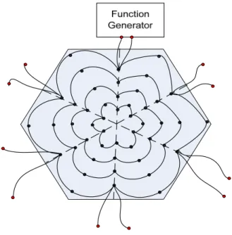
Based on the previous research done by Nur Azliza Ahmad from Universiti Teknologi PETRONAS on Development of a Powerful EM Transmitter [16], it is showing that hexagon shape is best design for a transmitter. The design that has been made was using one source and the copper winding made was in straight pattern as shown in Figure 9;
Figure 9: Hexagon transmitter with straight copper winding
13
3.3 Design Stage and Prototype Construction
Figure 10: How a wave launched by a Horn Transmitter [8]
Figure 11: How a wave launched by a Curve Transmitter [8]
In this project, the transmitter was designed based on the horn shape.
Referring on the literature review, it stated that the horn shape is classified as the aperture field radiation sources where both electric and magnetic fields across the horn’s aperture serve as the source of the radiated field which means, higher EM waves propagation produced.
The transmitter was also designed to be in hexagon shape with curve copper windings (6m) and has six supply sources (shown in Figure 14) compare to the previous design (Figure 9) which has straight copper windings and has only one supply source. The purpose of having the 6 curves winding shape is as it can provide a sharp and focus EM field. The winding wires was made from the copper since it is
14
a highly conductive material which then will governs to the bigger amount of induced current. Six supplies were connected to each 1m (six segments) of copper winding to create the constructive interference and this allows a higher EM waves transmission.
Figure 12: The Constructive Interference [17]
Whenever the EM field travelling along the rocks (where there are oil trapped) it will carry along the energy and this cause the oils trapped are going to vibrate and thus will help them to release from the rock and become as the droplets.
The skin depth theory is referred in order to know how much EM waves could penetrate and diffuse into the reservoir (see Figure 13).
15
Figure 13: Reservoir rocks have oil trapped in its pores
Figure 14: The Designed EM Transmitter which has six segments with 1m copper winding each. Each segment is connected to the 1 KHz frequency supply.
16 3.4 Experiment To Find The Recovery
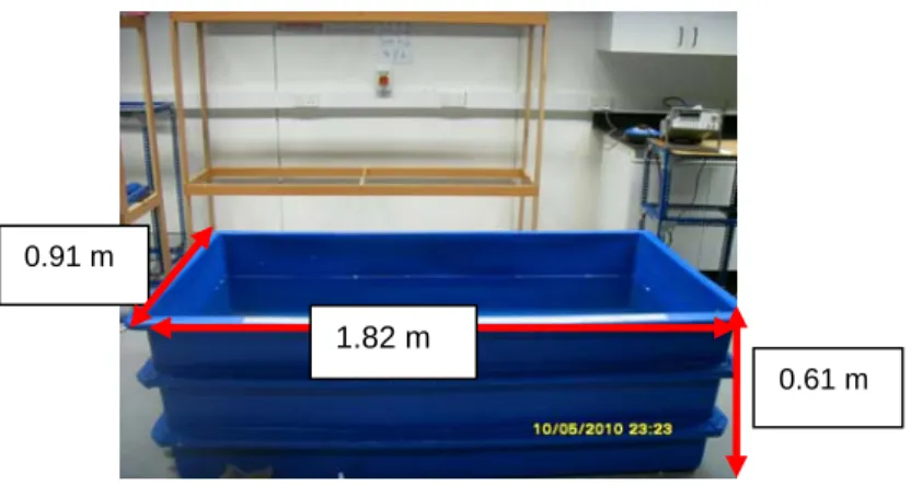
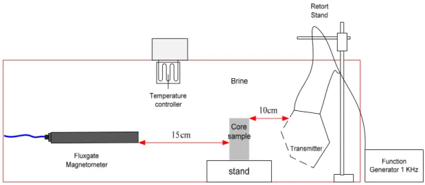
Figure 15: Schematic Diagram of the Experimental Setup 3.41 Tank
A tank with size of 1.92m X 0.91m X 0.61m was used with the temperature controller together.
Figure 16: Tank
1.82 m 0.91 m
0.61 m
17 3.42 Transmitters
The transmitter was fabricated using the copper-curve shape wires in a hexagon-shape prospect. Power amplifier and magnetic feeders were used in order to increase the EM waves transmitted. This transmitter was constructed with six segments from 6m of copper wire winding and with 6 sources.
Figure 17: The designed EM Transmitter 3.43 Brine
Brine (density is 1.0061g/cm3) water was used in order to conduct and allow the transmission of EM wave to the core rock.
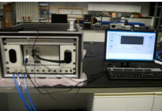
3.44 Data acquisition system (DAS) Model NI PXI-1042 (for EM data storage) and Fluxgate Magnetometer Model Bartington.
DAS and Fluxgate Magnetometer were used in order to detect and store the data of the EM waves that transmitted through the core rock.
15cm
15cm
18
Figure 18: Data acquisition system (DAS) is a product and/or processes used to collect information to document or analyze some phenomenon.
Figure 19: Fluxgate Magnetometer is capable of measuring the strength of any component of the Earth's magnetic field by simply re-orienting the instrument so that the cores are parallel to the desired component.
3.45 Temperature Controller
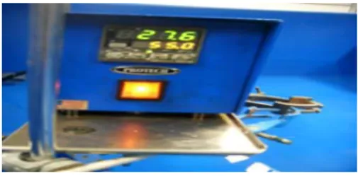
The temperature controller Protech SDC10 was used to maintain the temperature in order to get a reservoir-look-alike set up. The temperature in the tank for the experiments purpose is about 37ºC.
19
Figure 20: Protech SDC10 Temperature Controller is used to maintain the temperature of 0.91m x 1.82m x 0.61m tank to be around 37 0C 3.46 Function Generator
The 1 KHz function generator was used as the transmitter supply source and also as the supply to the magnetic feeder.
Figure 21: Function generator 5MHz model Instek GFG-8250A 3.47 DC Power Supply Model GPC-3030DQ
Dc power supply was used to supply the amplifier with 12V.
Figure 22: DC power supply
20 3.48 Amplifier
Power amplifier was used to increase or amplifies the amplitude of the signal which in this case, the current that flowing in the transmitter conductor.
Higher current will contribute to higher EM wave’s transmission. This amplifier is operated by supplying 12V DC supply and 1 KHz frequency.
Figure 23: Power Amplifier 3.49 Magnetic Feeder
Magnetic Feeder was used to increase amplitude of EM waves transmitted by the designed transmitter.
These feeders were prepared using sol gel method which resulted in getting nanoparticles. The nanoparticles were formed to toroid shaped sample with 0.5cm outer diameter and 0.25cm in height (refer to Table 1).
Figure 24: Nanoparticle Magnetic Feeder
21
Table 1: Magnetic feeder characteristics
Parameter 700° C 900° C
Weight (g) 0.5 0.5
Outer Diameter (cm) 0.5 0.5
Inner Diameter (cm) 0.25 0.25
Height (cm) 0.25 0.25
Density (g/cm3) 3.4 3.4
Number of winding 20 20
Material of winding Copper wire Copper wire
3.50 Core Rock samples
The core rock sample used has the below characteristics:
Table 2: Core Sample Characteristics Core rock with sample ID: A
Figure 25: The Core Sample
Length(mm): 73.66 Weight(g): 171.53 Diameter(mm): 38.02 Permeability: 567.8002 Vp(cc), Pore Volume: 17.7657 Φ(%), Porosity: 21.1771 Vgrain (g/cc): 66.1254 Vbulk(g/cc): 83.8910
22 3.51 Helium Porosimeter
Helium Pososimeter was used in order to analyze the main data measurements for the core sample which are the pore volume, porosity and permeability. Porosity is the percentage that the volume of the pore space bears to the total bulk volume, which is the pore space that determines the amount of space available for storage of fluids.
Pore volume is the volume of connected pores in a core sample in which the fluids can flow, and permeability is the ability of a rock to transmit fluid through the pore spaces.
Figure 26: Helium Porosimeter 3.52 Core Flooding Machine
Core flooding machine was used in order to prepare the core sample with the brine and also with the crude oil. For this purpose, a syringe pump introduces a fluid into the core holder (see Figure 28). The process of the flooding was involved with the used of injection of brine and crude oil at a high pressure
23
and low flow rates. For the data obtained from the core rock flooding, we can device the EM wave method to recover as much oil as possible.
Figure 27: The Core Flooding Machine
Figure 28: The Core Holder
24 3.53 Weighing Apparatus
The weighing apparatus was used to weight the core sample from time to time. The weighing apparatus with three decimal places was used in order to get more accurate measurements which are very important in the recovery calculation.
Figure 29: Weighing Apparatus 3.54 Caliper
Caliper was used to measure the height, wide and thickness of the core sample. These measurements are then used to the Helium Porosimeter in order to check their porosity, pore volume and permeability.
Figure 30: Caliper
25
3.55 CST (Computer Simulation Technology ) software
The electromagnetic simulation software CST STUDIO SUITE™ is the culmination of many years of research and development into the most efficient and accurate computational solutions to electromagnetic design. It comprises CST’s tools for the design and optimization of devices operating in a wide range of frequencies – static to optical. Analyses may include thermal and mechanical effects, as well as circuit simulation. All programs are accessible through a common interface with facilitates circuit and multi- physics co-simulation.
By using CST, the significant of transmitter’s shape can be analyzed based on the E-field and B-field produced.
26
CHAPTER 4
RESULTS AND DISCUSSION
Experiment 1: Simulation on Straight and Curve wire
Equipments and materials used: CST (Computer Simulation Technology) Description:
This simulation was done in order to see how the E-field and B-field transmitted pattern in straight and curve wire is looked like and thus to determine which pattern is the best in term of E-field and B-field to be the transmitter base. Straight aluminium wire (15.7cm long) and curve aluminium wire (15.7cm long and 10cm in diameter) were used. Both wire pattern were supplied with 1 KHz frequency and injected with 20 A of current.
27 Results:
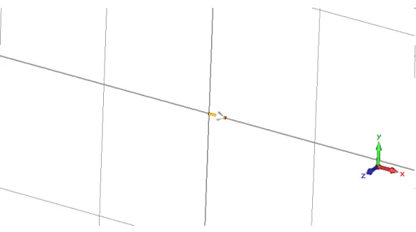
Figure 31: Current path in a 15.7cm straight Wire
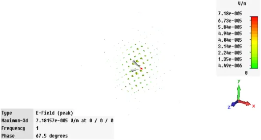
Figure 32: The electric field produced in Straight Wire (Maximum is 7.81e-005 Vs/m2)
28
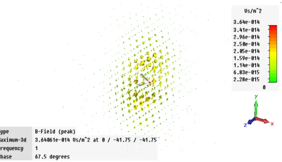
Figure 33: The magnetic field produced in Straight Wire (Maximum is 3.64e-14 Vs/m2)
Figure 34: Current Path in Curve Wire
29
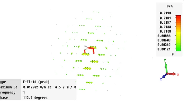
Figure 35: The electric field produced in Curve Wire (Maximum is 0.0193 V/m)
Figure 36: The magnetic field produced in Curve Wire (Maximum is 9.46e-11 Vs/m2)
30 Discussion and Conclusion:
From the simulation results shown, we could see that there are different patterns of how E-field and B-field distribution are. With curve aluminum wire, the B-field distribution is likely more focused rather than B-field in straight wire which is equally distributed. The characteristic of focused B-field with higher value compared to the straight wire is very important in order to design a good EM transmitter.
The electric field produced is higher in a curve wire compare to the straight wire with 99.6% of increment. Table 3 shows that the value of both B-field and E-field in curve wire is higher than in straight wire.
Table 3: B field and E field
Curve Wire Straight Wire
B field (T) 9.46e-11 3.64e-14
E field(V/m) 0.0193 7.81e-5
31
Experiment 2: Designing EM Transmitter Using CST
Equipments and materials used: CST (Computer Simulation Technology) Description:
This simulation was done in order to see the significant of having more aluminum wires instead of having just one wire as the transmitter base. The primary simulation was carried out by considering the straight aluminum wire instead of curve wire and to be understood that the results for curve wires would be exceeding base on the results in experiment 1.
The simulation was made with a 15cm straight aluminum wire. For this experiment, 80 MHz and 20A of current were supplied to the model. The aluminum wire numbers then were increased up to eight and the B-field distributions were recorded and analyzed.
32 Results:
Figure 37: Source Current in one straight wire
Figure 38: B-field distribution in one straight wire
33
Figure 39: Source Current in two straight wires
Figure 40: B-field distribution in two straight wires
34
Figure 41: Source Current in three straight wires
Figure 42: B-field distribution in three straight wires
35
Figure 43: Source Current in six straight wires
Figure 44: B-field distribution in six straight wires
36 Discussion and Conclusion:
Referring to the results of simulation done, the significant of having more aluminum wires are shown up to eight aluminum wires used where the B-field distribution is increasing proportional to the increment of the aluminum wires. However, the significant of having more wires are not applicable to the number of wire more than six where the value of B-field distribution is start to decrease.
The six straight wires give the highest value of magnetic field distribution which is 0.0015T.
Table 4 shows the data on B-field distribution for the numbers of aluminum wires used in this simulation.
Table 4: The distribution of B-field in one up to eight wires Number of straight wire B-field (T)
1 wire 0.00000155 2 wires 0.00041 3 wires 0.000397 4 wires 0.000520 5 wires 0.000632 6 wires 0.0015 7 wires 0.000861 8 wires 0.000797
37
Experiment 3: Experimental Work on the Significant of Supply Connection Equipments and materials used:
1. Function generator 5MHz
2. Straight aluminium rods (transmitter) with length of 15.7cm 3. Magnetic feeder with frequency supply equal to 1Khz 4. Fluxgate magnetometer
5. Wire clippers Description:
The purpose of this experiment done was to investigate the significant of having different type of supply connections which are series connection or parallel connection when having more than one wire in one time. Due to the availability of materials in lab, the experiment conducted was on the three straight aluminium rods with 15cm long and 1cm in diameter. In the first run, one straight rod with magnetic feeder was connected to the 5 MHz function generator and both were supplied with 1 KHz frequency. The rod with the magnetic feeder then left for about half an hour with the fluxgate magnetometer in order to get better and accurate data of B-field distribution by the straight rod aluminium. The fluxgate magnetometer was placed 30cm apart from the aluminium rod.
The experiment was furthered by considering two and three aluminium rods with magnetic feeder by applying both type of supply connections, series and parallel.
The B-field distribution produced by the aluminium rods then has been identified by the fluxgate magnetometer.
38 Figure 45
1 Straight rod
Figure 46
2 Straight rods with parallel supply
connection
Figure 47
3 Straight rods with parallel supply
connection
Magnetic feeder
Straight aluminum rod
Fluxgate magnetometer
30cm
39 Results:
Table 5: The average of magnetic field produced by 1 straight rod with a power source
1 rod _1 1 rod _2 1 rod _3 Ave 4.18E‐08 4.13E‐08 4.21E‐08 4.17E‐08 4.29E‐08 4.20E‐08 4.17E‐08 4.22E‐08 4.27E‐08 4.25E‐08 4.23E‐08 4.25E‐08 4.20E‐08 4.17E‐08 4.19E‐08 4.19E‐08 4.22E‐08 4.23E‐08 4.16E‐08 4.20E‐08 4.24E‐08 4.22E‐08 4.19E‐08 4.22E‐08 4.19E‐08 4.17E‐08 4.15E‐08 4.17E‐08 4.24E‐08 4.22E‐08 4.22E‐08 4.23E‐08 4.25E‐08 4.22E‐08 4.23E‐08 4.23E‐08 4.25E‐08 4.24E‐08 4.22E‐08 4.24E‐08 4.20E‐08 4.17E‐08 4.21E‐08 4.19E‐08 4.23E‐08 4.24E‐08 4.21E‐08 4.23E‐08 4.28E‐08 4.19E‐08 4.21E‐08 4.23E‐08 4.22E‐08 4.25E‐08 4.22E‐08 4.23E‐08 4.17E‐08 4.27E‐08 4.18E‐08 4.21E‐08
4.21E‐08
Table 6: The average of magnetic field produced by 2 straight rods with parallel power source
2 rods_dif source_1
2 rods_dif source_2
2rods_dif source_3
Ave
9.48E‐07 9.59E‐07 9.29E‐07 9.45E‐07 9.48E‐07 9.57E‐07 9.30E‐07 9.45E‐07 9.48E‐07 9.55E‐07 9.29E‐07 9.44E‐07 9.49E‐07 9.57E‐07 9.28E‐07 9.45E‐07 9.46E‐07 9.59E‐07 9.27E‐07 9.44E‐07 9.49E‐07 9.60E‐07 9.28E‐07 9.46E‐07 9.48E‐07 9.59E‐07 9.26E‐07 9.44E‐07 9.47E‐07 9.57E‐07 9.28E‐07 9.44E‐07 9.45E‐07 9.56E‐07 9.30E‐07 9.44E‐07 9.44E‐07 9.57E‐07 9.32E‐07 9.44E‐07
40
9.41E‐07 9.59E‐07 9.32E‐07 9.44E‐07 9.43E‐07 9.59E‐07 9.32E‐07 9.45E‐07 9.42E‐07 9.59E‐07 9.31E‐07 9.44E‐07 9.42E‐07 9.58E‐07 9.31E‐07 9.44E‐07 9.45E‐07 9.57E‐07 9.31E‐07 9.44E‐07
9.44E‐07
Table 7: The average of magnetic field produced by 3 straight rods with parallel power source
3 rods_dif source_1
3 rods_dif source_2
3 rods_dif source_3
Ave
1.57E‐06 1.56E‐06 1.57E‐06 1.56E‐06 1.56E‐06 1.57E‐06 1.56E‐06 1.56E‐06 1.57E‐06 1.57E‐06 1.57E‐06 1.57E‐06 1.57E‐06 1.56E‐06 1.57E‐06 1.56E‐06 1.57E‐06 1.57E‐06 1.57E‐06 1.57E‐06 1.56E‐06 1.57E‐06 1.56E‐06 1.56E‐06 1.57E‐06 1.56E‐06 1.57E‐06 1.57E‐06 1.56E‐06 1.57E‐06 1.57E‐06 1.57E‐06 1.56E‐06 1.57E‐06 1.56E‐06 1.56E‐06 1.57E‐06 1.56E‐06 1.57E‐06 1.57E‐06 1.56E‐06 1.57E‐06 1.57E‐06 1.57E‐06 1.57E‐06 1.57E‐06 1.56E‐06 1.56E‐06 1.57E‐06 1.56E‐06 1.57E‐06 1.57E‐06 1.56E‐06 1.56E‐06 1.57E‐06 1.56E‐06 1.57E‐06 1.57E‐06 1.56E‐06 1.56E‐06
1.56E‐06
41
Table 8: The average of magnetic field produced by 2 straight rods with series power source.
2 rods_series source_1
2 rods_series source_2
2 rods_series source_3
Ave
5.32E‐07 5.23E‐07 5.20E‐07 5.25E‐07 5.28E‐07 5.15E‐07 5.21E‐07 5.21E‐07 5.31E‐07 5.24E‐07 5.13E‐07 5.22E‐07 5.24E‐07 5.22E‐07 5.21E‐07 5.22E‐07 5.30E‐07 5.22E‐07 5.21E‐07 5.24E‐07 5.29E‐07 5.24E‐07 5.20E‐07 5.24E‐07 5.28E‐07 5.16E‐07 5.20E‐07 5.21E‐07 5.29E‐07 5.24E‐07 5.16E‐07 5.23E‐07 5.22E‐07 5.25E‐07 5.21E‐07 5.23E‐07 5.30E‐07 5.25E‐07 5.20E‐07 5.25E‐07 5.29E‐07 5.27E‐07 5.12E‐07 5.23E‐07 5.28E‐07 5.23E‐07 5.20E‐07 5.24E‐07 5.28E‐07 5.27E‐07 5.19E‐07 5.25E‐07 5.18E‐07 5.27E‐07 5.19E‐07 5.21E‐07 5.27E‐07 5.20E‐07 5.19E‐07 5.22E‐07
5.23E‐07
42
Table 9: The average of magnetic field produced by 3 straight rods with series power source
3 rods_series source_1
3 rods_series source_2
3 rods_series source_3
Ave
7.56E‐08 7.52E‐08 7.47E‐08 7.52E‐08 7.53E‐08 7.51E‐08 7.49E‐08 7.51E‐08 7.52E‐08 7.51E‐08 7.46E‐08 7.50E‐08 7.59E‐08 7.52E‐08 7.43E‐08 7.52E‐08 7.52E‐08 7.51E‐08 7.47E‐08 7.50E‐08 7.54E‐08 7.51E‐08 7.44E‐08 7.50E‐08 7.54E‐08 7.51E‐08 7.48E‐08 7.51E‐08 7.50E‐08 7.50E‐08 7.45E‐08 7.48E‐08 7.57E‐08 7.50E‐08 7.43E‐08 7.50E‐08 7.50E‐08 7.53E‐08 7.47E‐08 7.50E‐08 7.45E‐08 7.56E‐08 7.50E‐08 7.51E‐08 7.50E‐08 7.55E‐08 7.56E‐08 7.53E‐08 7.55E‐08 7.52E‐08 7.48E‐08 7.52E‐08 7.51E‐08 7.54E‐08 7.44E‐08 7.50E‐08 7.45E‐08 7.49E‐08 7.43E‐08 7.46E‐08
7.50E‐08
43 Discussion and conclusion:
Results in Table 5 to Table 9 were analyzed and plotted in the bar chart as shown in Figure 48. From the Figure 48, the three straight aluminium rods with parallel power source has the highest value of magnetic field produced (1.56E-6). Parallel connection produce higher magnetic field because the connection provides the interference of waves where in this case, constructive interference was occurred.
Two interfering waves have a displacement in the same direction and give a ‘super- crest’ which increase the value of magnetic field.
Figure 48: B-field for two source connection types
44
Experiment 4: Experimental Works on Aluminum Rod and Aluminum Wire Equipments and materials used:
1. Function generator 80MHz
2. Curve aluminium rod with diameter of 10cm without magnetic feeder 3. Curve aluminium wire with diameter 10 cm without magnetic feeder 4. Wire clippers
5. Oscilloscope
6. Magnetic feeder (as receiver) Description:
The fourth experiment was conducted in order to investigate the significant of material used for the transmitter design purpose which is between the aluminium rod and aluminium wire. For this experiment, aluminium curve rod (10cm diameter) and aluminium curve wire (10cm diameter) without magnetic feeder were used. Both were supplied with 80 MHz frequency. Oscilloscope was used to record the average received frequency that mostly appeared on the screen.
45 Results:
Table 10: Frequencies received by receiver for 1 curve aluminum rod and 1 curve aluminum wire (Frequencies are in MHz)
Readings 1 curve rod aluminum without m.feeder
1 curve aluminum wire without m.feeder
1 149.3 210.1
2 149.3 218.0
3 161.2 207.0
4 161.2 204.0
5 161.2 209.4
6 161.2 208.3
7 161.2 208.3
8 151.5 209.4
9 151.5 207.0
10 151.5 208.3
11 174.2 210.1
12 174.2 208.3
13 173.0 208.3
14 176.0 206.6
15 187.3 206.6
Average 162.9 208.6
Discussion and conclusion:
Based on the result in Table 10, with an aluminum curve wire without magnetic feeder, the value of frequency received is 208.6 MHz compare to aluminum rod, 162.9 MHz which shows that copper wire has a better ability to transmit higher frequency compared to the aluminum rod. This is due to the higher purity in aluminum wire rather than purity in aluminum rod.
The increment of frequency is about 28% if we use aluminum wire as the transmitter rather than aluminum rod.
Therefore, it was decided to design the transmitter in hexagon shape with the wire windings rather than to have transmitter with six connected rods.
46
Experiment 5: Experimental Work on More Aluminum Curve Wires Used Equipments and materials used:
1. Function generator 80MHz
2. Eight aluminium wires with diameter 10 cm without magnetic feeder 3. Wire clippers
4. Oscilloscope
5. Magnetic feeder (as receiver) Description:
Fifth experiment was done in order to figure out the ability of having more aluminium curve wires in increasing the value of transmitted frequency. In this experiment, 80 MHz frequency with parallel connection was supplied to the aluminium wires. The range of frequencies that mostly appeared on the oscilloscope was taken. 15 readings were recorded and the average of frequencies was calculated.
The aluminium curve wires used were up to eight in numbers.
47 Figure 49
1 aluminum wire
Figure 50
2 aluminum wires
Figure 51
3 aluminum wires 2 aluminum wires
3 aluminum wires
Receiver
48 Figure 52
4 aluminum wires
Figure 53
5 aluminum wires
Figure 54
6 aluminum wires 5 aluminum wires
4 aluminum wires
49 Figure 55
7 aluminum wires
Figure 56
8 aluminum wires
50 Result:
Table 11: Frequencies received by receiver for 1 until 8 curve aluminum wires (Frequencies are in MHz)
Readings 1 curve
2 curves
3 curves
4 curves
5 curves
6 curves
7 curves
8 curves 1 210.1 295.7 331.1 434 549.5 555.5 555.6 555.6 2 218 282.5 331.1 434 549.5 555.5 555.6 555.6 3 207 267.2 333.1 434 537.3 555.5 555.6 555.6 4 204 279.3 333.1 431.3 537.3 568.5 555.6 555.6 5 209.4 267.2 328.3 431.3 537.3 568.5 555.6 568.2 6 208.3 267.2 328.3 431.3 561.4 598.4 555.6 568.2 7 208.3 294.7 367 427 531.3 625 555.6 568.2 8 209.4 279.3 367 427 595.6 625 555.6 568.2 9 207 279.3 314.5 423.7 625 625 555.6 568.2 10 208.3 294.7 326.8 442.7 625 657 568.2 568.2 11 210.1 295.7 387 403 641.2 657 568.2 543.5 12 208.3 279.3 362.2 438.8 641.2 657 568.2 602.4 13 208.3 279.3 357.5 420 657.7 641.8 567.5 602.4 14 206.6 279.3 340 471 657.7 641.8 537 657.2 15 206.6 279.3 331.1 480 648 609 602 568.2 Average 208.6 281.3 342.54 435.3 593.0 609.4 560.8 573.7
51
Figure 57: The average frequency received Discussion and Conclusion:
From the results shown in Figure 57, the increment of received frequency for each increment of aluminum wire was about 22% to 35%. For example, by using one aluminum wire, the frequency received was 208.65 MHz and for two aluminum wires, the frequency received was 281.33 MHz which give about 34.5% of increment.
The relevant number of aluminum wire to be used based on the results is by having six aluminum wires because the frequency transmitted for more than six wires will be equally the same values; this is about 567.227 MHz in average.
52
Experiment 6: Experiment Work on Nanoparticle Magnetic Feeder and Amplifier.
Equipments and materials used:
1. Function generator 1KHz 2. Designed transmitter 3. Wire clippers
4. Fluxgate Magnetometer 5. Nanoparticle Magnetic feeder 6. Power amplifier
Description:
Further experiment was done in order to evaluate the significant of using nanoparticle magnetic feeder and amplifier with the designed EM transmitter in term of B-field transmitted. The experiments were done in three conditions;
I. Transmitter without amplifier and magnetic feeders II. Transmitter with amplifier
III. Transmitter with amplifier and magnetic feeders
For the first experiment the transmitter was connected in parallel connection with the 1 KHz frequency supply and left for 30 minutes. The fluxgate magnetometer was placed 25cm from the running transmitter and the B field transmitted data was saved and analyzed. The same procedures were considered for the other two conditions where amplifier and nanoparticle magnetic feeders were used.
Figure 58: Experiment Set up to Evaluate the EM Transmitter When Using NanoParticle Magnetic Feeders and Power Amplifier
EM Transmitter Fluxgate
Magnetometer
25 cm
53 Results:
Table 12: B field transmitted without amplifier and magnetic feeder
without Mf&_1
without Mf&_2
without Mf&_3
Average
4.08E‐09 4.13E‐09 4.02E‐09 4.07E‐09 4.42E‐09 4.01E‐09 4.27E‐09 4.23E‐09 4.13E‐09 3.97E‐09 4.25E‐09 4.11E‐09 4.33E‐09 4.18E‐09 4.32E‐09 4.27E‐09 4.64E‐09 3.67E‐09 4.47E‐09 4.26E‐09 4.07E‐09 4.46E‐09 4.13E‐09 4.22E‐09 4.26E‐09 4.19E‐09 3.84E‐09 4.09E‐09 4.28E‐09 4.09E‐09 4.29E‐09 4.22E‐09 4.07E‐09 4.07E‐09 4.39E‐09 4.18E‐09 4.34E‐09 4.14E‐09 4.33E‐09 4.27E‐09 4.36E‐09 4.22E‐09 4.20E‐09 4.26E‐09 4.02E‐09 4.29E‐09 3.94E‐09 4.09E‐09 3.84E‐09 4.34E‐09 4.69E‐09 4.29E‐09 4.21E‐09 4.17E‐09 4.52E‐09 4.30E‐09 4.26E‐09 4.10E‐09 4.13E‐09 4.16E‐09 3.99E‐09 4.41E‐09 4.45E‐09 4.28E‐09 4.16E‐09 4.21E‐09 4.51E‐09 4.30E‐09 4.01E‐09 4.29E‐09 4.53E‐09 4.28E‐09 4.13E‐09 4.75E‐09 4.41E‐09 4.43E‐09 4.39E‐09 4.37E‐09 4.22E‐09 4.33E‐09 4.65E‐09 4.05E‐09 4.45E‐09 4.38E‐09 4.46E‐09 4.10E‐09 4.31E‐09 4.29E‐09 4.26E‐09 4.46E‐09 4.15E‐09 4.29E‐09 4.21E‐09 4.22E‐09 4.11E‐09 4.18E‐09 4.26E‐09 3.84E‐09 4.00E‐09 4.03E‐09 4.37E‐09 4.17E‐09 4.32E‐09 4.28E‐09 4.14E‐09 3.82E‐09 4.47E‐09 4.14E‐09 4.22E‐09 4.62E‐09 4.23E‐09 4.36E‐09 4.32E‐09 4.42E‐09 4.57E‐09 4.43E‐09 4.40E‐09 4.30E‐09 3.95E‐09 4.22E‐09 4.30E‐09 4.19E‐09 4.59E‐09 4.36E‐09
4.25E‐09
54
Table 13: B field transmitted with amplifier
with amp_1 with amp_2 with amp_3 Average 5.22E‐09 6.39E‐09 6.04E‐09 5.88E‐09 6.02E‐09 5.78E‐09 6.43E‐09 6.08E‐09 6.12E‐09 4.63E‐09 6.07E‐09 5.61E‐09 6.37E‐09 3.43E‐09 4.84E‐09 4.88E‐09 5.17E‐09 2.35E‐09 3.96E‐09 3.83E‐09 4.03E‐09 3.10E‐09 2.83E‐09 3.32E‐09 2.53E‐09 4.23E‐09 2.72E‐09 3.16E‐09 3.01E‐09 5.16E‐09 3.94E‐09 4.04E‐09 3.80E‐09 5.93E‐09 5.76E‐09 5.16E‐09 4.97E‐09 6.13E‐09 6.00E‐09 5.70E‐09 6.43E‐09 6.54E‐09 6.48E‐09 6.48E‐09 6.29E‐09 5.99E‐09 6.43E‐09 6.24E‐09 6.39E‐09 4.57E‐09 5.71E‐09 5.56E‐09 5.58E‐09 3.59E‐09 4.64E‐09 4.60E‐09 4.95E‐09 2.32E‐09 3.56E‐09 3.61E‐09 2.80E‐09 2.86E‐09 2.38E‐09 2.68E‐09 2.11E‐09 4.23E‐09 3.15E‐09 3.16E‐09 4.05E‐09 5.22E‐09 4.30E‐09 4.52E‐09 4.71E‐09 5.86E‐09 5.76E‐09 5.44E‐09 5.60E‐09 6.24E‐09 6.00E‐09 5.95E‐09 6.42E‐09 6.15E‐09 6.10E‐09 6.22E‐09 6.34E‐09 5.76E‐09 6.36E‐09 6.15E‐09 5.96E‐09 4.56E‐09 5.19E‐09 5.24E‐09 4.84E‐09 3.52E‐09 4.34E‐09 4.23E‐09 3.94E‐09 2.59E‐09 2.57E‐09 3.03E‐09 2.75E‐09 2.83E‐09 2.86E‐09 2.81E‐09 2.99E‐09 4.29E‐09 3.41E‐09 3.56E‐09 4.21E‐09 5.34E‐09 4.71E‐09 4.75E‐09 5.38E‐09 6.13E‐09 5.41E‐09 5.64E‐09 6.05E‐09 6.22E‐09 6.30E‐09 6.19E‐09 6.05E‐09 6.20E‐09 6.19E‐09 6.15E‐09
4.83E‐09
55
Table 14: B field transmitted with feeders
with m.feeder_1 with m.feeder_2 with m.feeder_3 Average 2.06E‐08 3.04E‐08 2.26E‐08 2.45E‐08 2.62E‐08 3.23E‐08 2.91E‐08 2.92E‐08 3.57E‐08 3.20E‐08 3.31E‐08 3.36E‐08 3.58E‐08 2.65E‐08 3.41E‐08 3.22E‐08 3.07E‐08 2.23E‐08 3.19E‐08 2.83E‐08 2.22E‐08 2.71E‐08 2.96E‐08 2.63E‐08 2.77E‐08 3.78E‐08 2.73E‐08 3.09E‐08 4.06E‐08 4.65E‐08 2.07E‐08 3.59E‐08 4.42E‐08 4.79E‐08 3.20E‐08 4.13E‐08 4.12E‐08 4.58E‐08 3.96E‐08 4.22E‐08 3.23E‐08 3.95E‐08 4.71E‐08 3.96E‐08 2.88E‐08 3.36E‐08 5.56E‐08 3.93E‐08 4.62E‐08 3.53E‐08 5.73E‐08 4.62E‐08 5.15E‐08 5.18E‐08 5.44E‐08 5.26E‐08 5.12E‐08 6.03E‐08 4.67E‐08 5.27E‐08 4.21E‐08 6.57E‐08 3.83E‐08 4.87E‐08 3.27E‐08 6.69E‐08 4.13E‐08 4.70E‐08 4.53E‐08 6.33E‐08 6.52E‐08 5.79E‐08 5.72E‐08 4.75E‐08 8.37E‐08 6.28E‐08 5.77E‐08 4.26E‐08 9.40E‐08 6.48E‐08 5.40E‐08 5.72E‐08 1.00E‐07 7.04E‐08 4.41E‐08 7.81E‐08 1.01E‐07 7.44E‐08 4.08E‐08 8.95E‐08 9.27E‐08 7.43E‐08 6.24E‐08 8.92E‐08 7.22E‐08 7.46E‐08 6.84E‐08 8.28E‐08 5.57E‐08 6.90E‐08 6.91E‐08 7.21E‐08 6.35E‐08 6.82E‐08 6.44E‐08 5.50E‐08 7.96E‐08 6.63E‐08 4.40E‐08 6.56E‐08 8.61E‐08 6.52E‐08 6.73E‐08 8.99E‐08 8.55E‐08 8.09E‐08 8.58E‐08 1.04E‐07 7.78E‐08 8.91E‐08 9.21E‐08 1.10E‐07 6.18E‐08 8.80E‐08
5.34E‐08
56
Table 15: B field transmitted with amplifier and feeder
with feeder+amp_1
with feeder+amp_2
with feeder+amp_3
Average
9.03E‐09 9.19E‐09 9.23E‐09 9.15E‐09 9.35E‐09 9.22E‐09 8.83E‐09 9.14E‐09 9.82E‐09 9.42E‐09 8.67E‐09 9.30E‐09 9.10E‐09 9.26E‐09 8.58E‐09 8.98E‐09 8.72E‐09 8.57E‐09 7.42E‐09 8.24E‐09 8.59E‐09 8.33E‐09 7.33E‐09 8.08E‐09 7.92E‐09 8.14E‐09 7.26E‐09 7.77E‐09 7.86E‐09 7.86E‐09 7.45E‐09 7.72E‐09 7.20E‐09 7.05E‐09 7.62E‐09 7.29E‐09 7.42E‐09 7.27E‐09 7.29E‐09 7.33E‐09 7.13E‐09 7.15E‐09 8.65E‐09 7.65E‐09 7.41E‐09 7.85E‐09 8.41E‐09 7.89E‐09 7.94E‐09 8.85E‐09 8.78E‐09 8.53E‐09 8.57E‐09 9.08E‐09 8.83E‐09 8.82E‐09 8.77E‐09 9.14E‐09 9.08E‐09 8.99E‐09 9.43E‐09 9.16E‐09 9.15E‐09 9.25E‐09 9.28E‐09 9.88E‐09 8.92E‐09 9.36E‐09 9.12E‐09 8.99E‐09 9.09E‐09 9.07E‐09 8.95E‐09 9.18E‐09 8.72E‐09 8.95E‐09 9.31E‐09 8.35E‐09 8.45E‐09 8.70E‐09 8.85E‐09 7.64E‐09 8.29E‐09 8.26E‐09 8.45E‐09 8.17E‐09 7.82E‐09 8.15E‐09 8.18E‐09 7.34E‐09 7.44E‐09 7.65E‐09 7.87E‐09 7.38E‐09 7.12E‐09 7.45E‐09 7.24E‐09 7.28E‐09 7.12E‐09 7.21E‐09 7.00E‐09 7.83E‐09 7.42E‐09 7.42E‐09 7.61E‐09 8.49E‐09 7.98E‐09 8.03E‐09 7.55E‐09 8.68E‐09 8.05E‐09 8.09E‐09 7.82E‐09 9.40E‐09 8.28E‐09 8.50E‐09 8.57E‐09 9.39E‐09 9.39E‐09 9.12E‐09 8.63E‐09 9.18E‐09 9.01E‐09 8.94E‐09
8.36E‐09
57 Discussion and Conclusion:
Figure 59: B field transmitted (T)
Figure 60: B field distribution (%)
58
From the results shown in the Figure 59, the transmitter’s B-field distribution is higher with the existence of the amplifier and nanoparticle magnetic feeders, where the transmitter’s B-field is increased by 96.7%. The B-field of the transmitter was increased because the amplifier has amplifies the current flow in the copper conductor wire which then govern to the higher B-field production, while the magnetic feeders are function as an additive to the additional of B-field produced by the transmitter.
From Figure 59 transmitter with nanoparticle magnetic feeders shows the increment about 25.6% while transmitter with amplifier has the increment of 13.67%. This is show that nanoparticle magnetic feeders and amplifier are suitable to be used with the transmitter.
Figure 60 shows by the percentage representation that the increment of magnetic field strength is the highest when we use magnetic feeders together with the amplifier.
59
Experiment 7: Porosity and Permeability Test for Core Sample.
Equipments and materials used:
1. Helium Porosimeter 2. Weighing Apparatus 3. Caliper
Description:
This experiment was conducted in order to evaluate the core sample characteristic which are included the porosity, pore volume and also the permeability. The core sample which was firstly has been measured its wide, height, thickness and weight (using calliper), was then placed into the porosimeter holder. Helium gas has been applied with high pressure and then all the data were taken after 30 minutes running the test.
60 Result:
Table 16: Measurements from Porosity Test
Data Measurement
Air Permeability(mD) 567.80 Pore Volume (cc) 17.77
Porosity (%) 21.18
grain Volume(cc) 66.13 bulk Volume(cc) 83.89 grain density(g/cc) 2.59 bulk density (g/cc) 2.04
Discussion and Conclusion:
These measurements are very important in order to investigate and understand about the relationship of porosity, pore volume and permeability with the oil recovery calculation. Higher pore volume would cause to the bigger volume of the connected pores in the core sample which means that more crude oil can be placed inside compared to the smaller pore volume.
61 Experiment 8: Core Flooding
Equipments and materials used:
1. Core Flooding Machine 2. Weighing Apparatus
3. Crude Oil with density of 0.811g/cc 4. Brine Water with density of 1.018g/cc Description:
This experiment was conducted in order to prepare the core sample with the crude oil and brine. There were four main processes that involved in this experiment. The first process was to be the saturation of the core sample with the brine water for 24 hours.
This procedure’s purpose was to make the core sample was fully saturated with the brine and to ensure that there was no air inside the core.
The other three processes were carried in the core flooding machine where the second process was about to have second brine water injection into the core sample.
Third process was to be the crude oil injection and fourth process was again the brine water injection. Figure 61 shows the parameter involved while doing this experiment where the inlet part was used to inject the brine and crude oil. Figure 61 also shows the pressure and temperature involved while preparing the core sample with brine and crude oil.
62
Figure 61: Parameters involved in Core Flooding Process Results:
Figure 62: Brine Water after Crude Oil Injection Inlet Outlet
Core Holder Overburden Pressure,
1443.6 psi
Core Temperature, 39 0C
63
Figure 63: Brine water after Second Brine Water Injection Process Table 17: Core Flooding OOIP and ROIP
Data Measurement
Porosity (%) 21.18 Pore Volume (cc) 17.77
OOIP (ml) 12
ROIP (ml) 6.2
64 Result and Discussion:
Second brine injection in the core sample using the Core Flooding Machine was to confirm that there was no air at all inside the core. Another purpose of having second brine water injection was as a measurement purpose to calculate the crude oil that would be placed inside the core sample where the volume crude oil placed in the core sample in the third process would be the same as the volume of brine water that came out from the outlet (see figure 62). The oil placed inside the core sample at this process was called as the Original Oil In place (OOIP).
The third brine injection purpose was to put the core rock into the real situation where the real reservoir would consist of crude oil with the brine water. In this process, the injection of brine water was stopped once we notice that there was no more oil coming out from the outlet part. The remaining oil inside the core sample was calculated and the called as the Residue Oil In Place (ROIP). ROIP was calculated by subtracting the water displacement after the process of brine injection from the OOIP volume (see Figure 63).
Table 17 shows that the value of OOIP and ROIP measurements.
65 Experiment 9: Oil Recovery Using EM waves Equipments and materials used:
1. 5 MHz function generator 2. DC power supply
3. Power Amplifier 4. Temperature controller 5. Weighing apparatus 6. Tank
7. Fluxgate Magnetometer Description:
This experiment was carried out in order to calculate the oil recovery by using the EM waves method where the designed EM Transmitter become the main tool to have the recovery. The experiment setup is shown in Figure 64. The core sample was left to be exposed to the EM waves for 36 hours where the weight of core sample was taken at 2,4,10,12,18,24 and 36 hours.
66 Set Up:
Figure 64: Experiment set up for oil recovery Result and Discussion:
This experiment was consist of two main parts which were including the analysis used to prove that the fluxgate magnetometer could be one of the calculation method of the recovery using EM waves and the another part was the analysis about the oil recovery.
The analysis in the oil recovery was then divided into two parts which were the analysis from the fluxgate magnetometer data and second part was the analysis from the core sample weight measurements. Both methods of recovery gave approximately the same values of recovery percentage.
Temperature controller
Fluxgate magnetometer Core
sample Transmitter
1 KHz source
10cm 25cm
67
Part 1: To Prove the Potential of Fluxgate Magnetometer to be a Tool of Oil Recovery Calculation.
Table 18: B field distribution in three conditions
without_c.Rock empty_c.Rock flooded_c.Rock(Ave)
2.71E‐08 2.72E‐08 4.5E‐08
Figure 65: B field distribution in three conditions
The B field transmitted by the transmitter was evaluated base on three conditions which are included;
a. B field propagation direct to the fluxgate magnetometer (without core rock)
b. B field propagation through the empty core sample (no crude oil and brine inside)
68
c. B field propagation through the flooded core sample (with crude oil and brine inside).
From Figure 65, we could see that the intensity of B field for both conditions without and with empty core rock is the same while intensity of B field through the flooded core rock was slightly higher than the other conditions. The increment on the B-field measurement shows that Fluxgate magnetometer could detect the crude oil inside core rock samples and can be a tool to calculate the oil recovery using EM waves.
Part 2: Analysis on the Oil Recovery
Figure 66: Core sample without oil droplet but with oily surface
After 12 hours
69
Figure 67: Core Sample with a little oil droplets
After 18 hours
Figure 68: Core sample with More Oil Droplets
After 24 hours
![Figure 12: The Constructive Interference [17]](https://thumb-ap.123doks.com/thumbv2/azpdforg/11084763.0/14.918.290.725.280.541/figure-12-the-constructive-interference-17.webp)