1 DESIGN OF A CONTROLLER FOR CAR SUSPENSION SYSTEM VIA STATE
SPACE APPROACH
By
SHARIFAH HANISAH BT SYED MOHD KHALID
Dessertation submitted in partial fulfilment of the requirements for the
Bachelor of Engineering (Hons) (Electrical Engineering)
AUGUST 2012
Universiti Teknologi PETRONAS Bandar Seri Iskandar
31750 Tronoh Perak Darul Ridzuan
Copyright 2012 by
Sharifah Hanisah bt Syed Mohd Khalid
2 CERTIFICATION OF APPROVAL
DESIGN OF A CONTROLLER FOR CAR SUSPENSION SYSTEM VIA STATE SPACE APPROACH
by
Sharifah Hanisah bt Syed Mohd Khalid
A project dissertation submitted to the
Department of Electrical & Electronic Engineering Universiti Teknologi PETRONAS
in partial fulfilment of the requirement for the Bachelor of Engineering (Hons) (Electrical & Electronic Engineering)
Approved:
__________________________
Assoc. Prof. Dr. Nordin Bin Saad Project Supervisor
UNIVERSITI TEKNOLOGI PETRONAS TRONOH, PERAK
AUGUST 2012
3 CERTIFICATION OF ORIGINALITY
This is to certify that I am responsible for the work submitted in this project, that the original work is my own except as specified in the references and acknowledgements, and that the original work contained herein have not been undertaken or done by unspecified sources or persons.
_______________________
[SHARIFAH HANISAH BT SYED MOHD KHALID 12440]
4
ABSTRACT
When it come to automobile performance, people will normally think about horse power torque and zero-to -60 acceleration. However with a good power generated by the piston engine it is still useless if the driver cannot manage to control the car. On the other hand, a good car performance will come together with a good suspension controlling. The propose of car suspension system is to minimize the friction between the tires and the road surface, to provide steering stability with good handling and having a comfort ride.
In this project , a brief information about car suspension system and how it work will be presented. In addition , state space approach have been chose for the method in the derivation of the mathematical modeling in designing controller to improve the performance of the suspension system.
Besides that, the controller design method using MATLAB software are also presented. The simulation result will help in analyzing the characteristic of the system and also be discussed to prove the controlling effects of the suspension system.
5 LIST OF TABLE
CHAPTER 1 INTRODUCTION ………1
1.1 Background ………1
1.2 Problem Statement ………2
1.3 Objectives ………3
1.4 Scope of Study ………3
CHAPTER 2 LITERATURE REVIEW ………4
2.1 Semi-Active suspension ……….………....……4
2.2 Passive suspension ……….5
2.2 Controllability and Observability...…...6
2.3 State space controller ………..………...6
CHAPTER 3 METHODOLOGY ……….…..7
3.1 Project Flow Chart ………….……….…….7
3.2 Tools and Equipment …….………..8
3.3 Gantt Chart ………...……….…9
CHAPTER 4: RESULT AND DISCUSSION 4.1 Introduction...10
4.2 Mathematical Modeling………...…11
4.3 System Responses……...………...…...17
4.4 State space Controller design……...………....20
4.41ntroduction...20
4.42 Feedback Controller...24
4.42 Feedforward Controller...30
4.5 PID Controller Design...45
4.51 Introduction...45
4.52 Tuning PID controller...46
4.53 Ziegler Nichols tuning method: closed loop...47
6
CHAPTER 5 CONCLUSION ………..…....57
5.1 Introduction...57
5.2 Conclusion...57
5.3 Suggestion for future work...58
7 LIST OF FIGURE
Figure 2.1: Semi-active car suspension ……….……….…..4
Figure 2.2: Passive car suspension...5
Figure 3.1 : Project Flow ...7
Figure 3.2 : Tools ...8
Figure 4.1: Passive suspension system ...11
Figure4.2 : Free body diagram for Sprun g...12
Figure 4.3: Free body diagram for Unsprung...14
Figure 4.4 Syetem Step Response ...18
Figure 4.5: Situation to simulate ...21
Figure 4.6 : Block diagram simulation model without controller...22
Figure 4.7 : result for state space mode ...22
Figure 4.8 : result for block simulation of the model XB ……….… 23
Figure 4.9 : Full Feedback Controller……….….24
Figure 4.10 : Simulation block diagram with feedback controller………..25
Figure 4.11: Result for k = 7.8870 -1.1222 5.8773 0.0085………..……..27
Figure 4.12: Result for k = 6.4211 -1.3677 6.4264 0.0038……….28
Figure 4.13: Comparison result for value K1 and K2 . ...28
Figure 4.14: Full Feed forward Controller………..30
Figure 4.15 : Simulation block diagram with feed forward controller………31
Figure 4.16: Result for Nr =14.7643………38
Figure 4.17: Result for Nr =13.8475………..………..…39
Figure 4.18: Result for Nr =0.2243………..………40
8
Figure 4.19: Result for Nr =25.1156………...….……41
Figure 4.20: Result for Nr = 2.3601………...…42
Figure 4.21: Comparison result for different value of Nr, feed forward gain……....…..43
Figure 4.22: Block Diagram for PID controller ...46
Figure 4.23: Block diagarm for PID controller ...48
Figure 4.24 : Closed loop unit step response (kc= 0.007) for sustained oscillation ...49
Figure 4.25 : Closed loop unit step response (kc= 0.00001) for sustained oscillation...49
Figure 4.26 : step response result for P controller...51
Figure 4.27 : step response result for PI controller...52
Figure 4.28 : step response result for PID controller...53
Figure 4.29 : Comparison step response between P, PI and PID controller ...54
Figure 4.30 : Comparison step response betwn PID controller n state space controller...56
9 LIST OF TABLE
Table 3.1 : Project Gantt chart………....………...9
Table 4.1 : Term and defination for Passive suspession Modeling………...11
Table 4.2 : Car suspension parameters………..………..…20
Table 4.3 : Comparison of step response with diffrent value of feedforward gain... 44
Table 4.4 : Zeigler –Nichols tuning rules...47
Table 4.5 :Zeigler-Nichols tuning values...50
Table 4.6 : comparison step response parameter for P, PI and PID controller...54
Table 4.7 : Comparison step response between PID controller and state space controller..56
10
1
CHAPTER 1 INTPRODUCTION
1.1 BACKGROUND
A car chassis comprises all the important system located under the car body ans suspension is one of it. Others main part of chassis are, the steering system, tires and the frame. Suspension system is basically connecting the wheels of the car to the car body.
When a car hits a bump or hit a hole on the road, it will experience jolts and this
suspension system will act as a body cushioned to give a stable and comfort ride.Besides that, this system are meant to support the vehicle weight, to maintains the body at relatively constant height , and to maintain the traction force between the tire and the road surface.
There are three type of car suspension system :
Passive suspension system
Semi- active suspension system
Active suspension system
Passive show that the suspension elements cannot supply energy to the
suspension system. This system includes the tradisional springs and shock absorbers. It has the ability to store energy using spring and dissipate the energy using the dampers.
Semi- active suspension system can control the dissipation of energy. In this system, controlled damper or semi -active damper under closed loop control is needed to regulate damping force by dissipate the energy.
In this project, state space approach use for designing and modeling the
controller for semi –active suspension system. The controller need to able to control the
2 relative motion between car body and wheels. Others than, overall performance of a semi- active suspension system will be determine. Result from this, will be compare with the passive system using MATLAB simulink.
1.2 PROBLEM STATEMENT
The primary goal for a semi- active suspension design is to find a solution for good ride quality, handling performance and suspension travel. When a car hit a bumps or a hole, it experiance vertical accelaration that will lower down car handling an comfort. Thus to reduce the vertical acceleration of the car body is the main function of suspension. A good suspension should have the ability to behave differently on smooth and rough roads, in order to enhance passenger comfort the desired response should be soft in the other hand suspension should stiffen up to avoid hitting its limit when the road surface is to rough.
However, this system ia a nonliner and unstable system, in such it providing a challenge to the control engineer or reseacrhers. Thus many efforts, approach and method that have been done to develop the controller for this system, yet there is no result for the best system approach.
.
3 1.3 OBJECTIVES
To give a good comfort ride and a good car handling experience
To model quarter car system using state space
To design a suitable controller and for suspension system
To simulate the design and analyze the best parameter for the system
1.4 SCOPE OF STUDY
This project scope of study is about the construction of the mathematical modeling for semi- active and passive suspension system for a quarter car model.
Then proceed with the designing the controller for both o the system using state space approach. MATLAB software will be used to simulate the result, and the result will be analyze and compare to find the best controller for the systems.
4
CHAPTER 2
LITERATURE REVIEW
2.1 Semi –Active suspension system
The diffrent between semi active and passive susupension system is the controlable damper. This system can provide real time dissipation of energy or can be said as rapid change in rat eof spring damping coeeficient. The controller can detemine the level of damping based on control strategy used by adjusting the damper into disired value.
Figure 2.1: Semi-active car suspension 1
5 2.2 Passive Suspension System
For Passive suspension system its contains, spring and damper where spring absorb the energy and damper dissipate the energy. The spring located parallel with the damper placed at each corner of the vehicle, and the combination of spring-damper in this class is called a “strut”[5] . To support the strut some additional element or special geometrical arrangement are also used to upgrade the performance of passive system.
For example, to increase the stiffness to roll motion, an additional roll spring (anti-roll bars )can be used. Trailing arms could be implemented between the sprung mass and the wheel hubs to reduce the dive and squat motion of the vehicle body during braking and acceleration.[5].
Figure 2.2: Passive car suspension
6 2.3 Controllability and Observability
The original theoretical concepts of controllability and observability was introduced by R. Kalma in 1960 are particularly important for practical implementation[6].
Controllability mean that a system is controllable where the system state can be change under control input. In the other hand, observability mean in order to see what going on inside the system under observation, the system must be observable[6].A linear
controllable system may be define as a system which can be steered to any state from the zero to initial state. Kalman‟s canonical decomposition provides the basic theory and computational algorithm to remove unnecessary state from a realization, while preserving the input output[6].
2.4 State space controller
In 1997, Carneige Mellon from University of Michigan had develop a procedure of designing state space controller in MATLAB for bus suspension system, [2]. The proposed method was applied to a suspension system, and simulation results show that substantial improvement in the performance was achieved compared with other local observer. An active suspension system gives better performance in term of comfort ride compared to passive suspension system was proved by study conducted by Yahya md.
Sam[3][4]. An active system also proves to increases a tires to road contact in order to make the vehicle more stable.
7
CHAPTER 3 METHODOLOGY
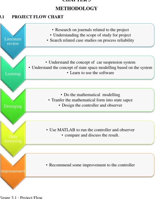
3.1 PROJECT FLOW CHART
Figure 3.1 : Project Flow Literature
review
• Research on journals related to the project
• Understanding the scope of study for project
• Search related case studies on process reliability
Learning
• Understand the concept of car suspension system
• Understand the concept of state space modelling based on the system
• Learn to use the software
Desinging
• Do the mathematical modelling
• Tranfer the mathematical form into state sapce
• Design the controller and observer
Data Analyzing
• Use MATLAB to run the controller and observer
• compare and discuss the result.
Improvement
• Recommend some improvement to the controller
8 3.2 TOOLS AND EQUIPMENT
MATLAB Software for data analysis and comparison
Microsoft Word - report writing
Figure 3.2 : Tools
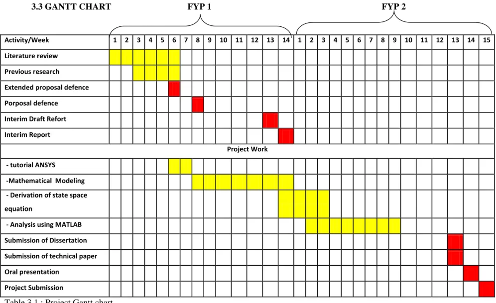
9 3.3 GANTT CHART FYP 1 FYP 2
Table 3.1 : Project Gantt chart
Activity/Week 1 2 3 4 5 6 7 8 9 10 11 12 13 14 1 2 3 4 5 6 7 8 9 10 11 12 13 14 15 Literature review Previous research Extended proposal defence
Porposal defence
Interim Draft Refort
Interim Report
Project Work
- tutorial ANSYS -Mathematical Modeling - Derivation of state space
equation
- Analysis using MATLAB Submission of Dissertation Submission of technical paper Oral presentation Project Submission
10
CHAPTER 4
RESULT AND DISCUSSION
4.1 Introduction
The main purpose of mathematical modeling is to obtain a state space representation of the quarter car model. This mathematical model allow to describe the relationship between the input and output, enable one to understand the behavior of the system.
A dynamic system can be describe by differential equation presentation via state space modelling. It use 1st order differential system. The state variables of a dynamic system are the variables making up the smallest set of variables that determine the state of the dynamic system. If at least n variables x1, x2… xn are needed to completely describe the behavior of a dynamic system (so that once the input is given for and the initial state at is specified, the future state of the system is completely determined), then such n variables are a set of state variables. ( Margaret Galvin, 2005) As for that, the state variables must not be physically measurable quantities. State variables must be choose in term of variables that do not represent physical quantities and those that are not measurable. It is an advantage of the state space methods where state variables can be freely choose. (Durbin and Koopman, 2004).
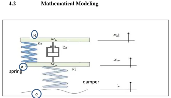
11 4.2 Mathematical Modeling
Figure 4.1: Passive suspension system
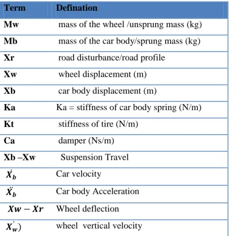
Refer to the figure 4.1, all the term use in the diagram can be define in the table below:
Table 4.1 : Term and defination for Passive suspession Modeling
Term Defination
Mw mass of the wheel /unsprung mass (kg) Mb mass of the car body/sprung mass (kg) Xr road disturbance/road profile
Xw wheel displacement (m) Xb car body displacement (m)
Ka Ka = stiffness of car body spring (N/m) Kt stiffness of tire (N/m)
Ca damper (Ns/m)
Xb –Xw Suspension Travel
̇ Car velocity
̈ Car body Acceleration Wheel deflection ̇ wheel vertical velocity
spring
damper B
A
G
12 From the figure 4.1, passive suspension system can be model by separating the body part and
tire part. The two masses are connected together by a suspension that is made up of a spring of stiffness Ks and absorber having a damping factor Cs.Each part, will have it own free body diagram, where every force acting in the parts can be classified. For this passive suspension system, the modeling analysis start with the free body diagram at the body part (sprung mass.).
( ( ̇ ̇ ̈ ……… (1) ̇ ̇ ̈
̈ ̇ ̇ Dividing equation (1) by , we get,
̈ ̇ ̇
( Figure4.2 : Free body diagram for Sprun g
14 Now, it‟s for Unsprung mass.
( ( ( ̇ ̇ ̈
̇ ̇ ̈ (
̈ ̇ ̇
̈ ( ̇ ̇
Dividing equation (2) by , we get, Figure 4.3: Free body diagram for Unsprung
15
̈ ( ̇ ̇
(
The state space equation can be written as:
̇ ̇
Thus, in state space the equation can be write as
̇ ̇
̇ ̈
̇
̇
̇ ̇
̇ ̈
(̇
̇
16
[ ̇̈̇
̈ ]
[
(
]
[
̇
̇ ]
[ ]
[ ] [
̇
̇ ]
[ ] [ ]
̇
̇ [ ̇̈̇
̈ ]
[
̇
̇ ]
[
(
]
[ ]
[ ]
17 and are the vertical displacement of mechanical point B, (Car body), and A (wheel) respectively, relatively to the initial position , and Xr is the ground reaction(given by the height of the road profile). Ka and Kt are the spring constant of the car and tyre and care represent the constant of the car shock absorber.
Thus, in this sub chapter, the system for quarter car modelling have been develop . A definite between input and output for quarter car model have been obtain using state space, thus, complete one of the objective of this project. Equation obtained will be used to simulate the system responses in following chapter.
4.3 System Responses
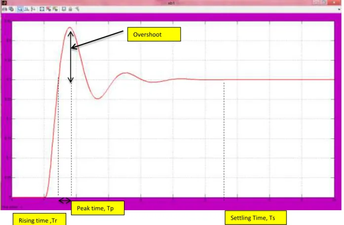
Usually road surfaces vary from one to another, it sometime can be bumpy and sometimes there are hole in it. Thus when a car pass through the bumper or the holes the excitation input „Step Response‟ which leads to vertical vibrations in car. In result of that, various shock absorbers were design to restore the steady state position of the car in the shortest possible time. Settling time is known as the time which the system takes to attain steady state equilibrium position is very important as the shorter the settling time, the more stable is the system. Figure 4.4 below shown the important parameters which will be used to analyse the result later.
18 Rising Time, Tr
Rising time is amount of time that the system takes to reach around 90% of its new set point.
Settling Time, Ts
Settling time is the time system takes to reach equilibrium to some level
Rising time ,Tr Settling Time, Ts
Peak time, Tp
Overshoot
Figure 4.4 Syetem Step Response
19 Peak Time, Tp
Peak time is the time that requires the system to reach the maximum overshoots point
Over shoot,
This is the maximum distance beyond the final value that the response reaches. It is usually expressed as a percentage of different between the original value and the final steady state value.
Steady state error
This is measure of how far the final value reached in the step response is from the actual desired value.
Thus in the next sub topic, controller for the system will be design via state space using several values of gain that will be obtain. Comparison of step response result among all the gain values will be done, and one of the gain value will choose as the best controller as it give the best result in the step response system.
20
4.4 State Space Controller Design 4.41 Introduction
First a verification of important property is needed, in order to apply state-space controller design techniques ,which is controllability. It is necessary to have this controllability property in corresponds to the ability to place the closed-loop poles of the system anywhere in the complex s-plane.
For the system to be completely state controllable, the controllability matrix [ | | | |]
must have rank n. The rank of a matrix is the number of independent rows . The number n corresponds to the number of state variables of the system. Adding additional terms to the controllability matrix with higher powers of the matrix A will not increase the rank of the controllability matrix since these additional terms will just be linear combinations of the earlier terms.
Since the model controllability matrix is 4x4, the rank of the matrix must be 4. The MATLAB command rank can give you the rank of this matrix.
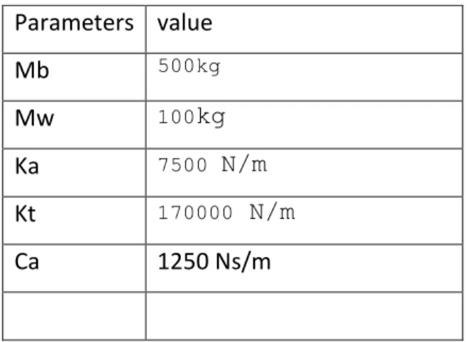
However before proceed with the system controllability, let list down all the parameters.
Parameters value
Mb 500kg
Mw 100kg
Ka 7500 N/m Kt 170000 N/m
Ca 1250 Ns/m
Table 4.2 : Car suspension parameters
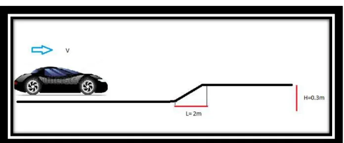
21 The reference Xr for the simulation refelects the road profile. For a road of 50m length , assuming the obstacle occur after 10m and the car speed is v=10m/s, the following define the corresponding reference input:
V= 10m/s L= 2m H = 0.3m
The MATLAB command rank can give you the rank of this matrix. Refer appendix for matlab coding for the matrix.
co = ctrb(A,B);
>> Controllability = rank(co) Controllability =
4
From the matlab, the system is completely state controllable since the controllability matrix has rank 4.
Figure 4.5: Situation to simulate
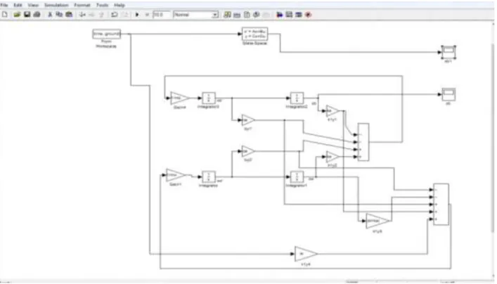
22 Below is the block diagram for quarter car suspension model. Let see how this
suspension model run without controller.
.
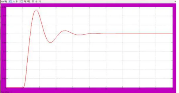
Figure 4.7 : result for state space model simulation XB1 Figure 4.6 : Block diagram simulation model without controller
Figure 4.7 : result for state space mode
23 Figure 4.8 : result for block simulation of the model XB
For XB n XB1, the result is the same, this mean, my block simulation that I build is correct since the result is same with the state space block from matlab. From the graph we can calculate rise time, settling time and overshoot of the system. This calculation result later will be compare with the result after applying the controller.
Rise time,
Peak = 0.433m Settling Time,
Overshoot%
24 4.42 Feedback Controller
In typical feedback control system the output y, is feedback to the summing junction. It is now the topology of design changes. Instead of feeding back y, it will then feedback all the state variable. If each state variable is feedback to the control u, through a gain K, there would be n gain that could be adjust to yield the required closed loop pole values. The feedback through the gain k is represent in figure by feedback vector K.
The new state equation for closed-loop system can be write as
̇ ( (
The stability and time domain performance of the closed-loop feedback system are determined primarily by the location of the poles (eigenvalues) of the matrix (A-BK).
Since the matrices A and B*K are both 4 by 4 matrices, there will be 3 poles for the system. By choosing an appropriate K matrix we can place these closed-loop poles Figure 4.9 : Full Feedback Controller
25 anywhere we want. We can use the MATLAB function placeto find the control matrix, K, which will give the desired poles.
Before attempting this method, we have to decide where we want the closed-loop poles to be.
Using mat lab command , the eigen value of the system can be determine.
Below is the simulation block diagram with feedback controller in matlab
Figure 4.10 : Simulation block diagram with feedback controller
26 Thus to obtain gain K, we need to adjust these poles value to desired value which
approaching the left of s-lane. The desired pole values that been chose are:
Value 1
p1 = -12.3 +82i p2= -12.3 - 82i p3 = -2.4 +7i p4= -2.4 -7i
From this value, matrix gain can be obtain by this matlab command.
k = place(A,B, [p1 p2 p3 p4])
k = 7.8870 -1.1222 5.8773 0.0085
Then , putting all the feedback gain value1 in the system model simulation, we can see the result in figure 4.10:
27 Figure 4.11: Result for k = 7.8870 -1.1222 5.8773 0.0085
Value 2 p1= -9+82i;
p2= -9 - 82i;
p3= -1.7 +7i;
p4= -1.7 - 7i;
From this value, matrix gain can be obtain by this matlab command k = place(A,B, [p1 p2 p3 p4])
k =
6.4211 -1.3677 6.4264 0.0038
28 Then , putting all the feedback gain value 2 in the system model simulation, we can see the result in figure 4.11.
Figure 4.12: Result for k = 6.4211 -1.3677 6.4264 0.0038 The comparison of gain 1 and gain 2,
Figure 4.13: Comparison result for value K1 and K2
29 From figure 4.12 we can see that gain 1 give better result since . Controller with gain 2 have less overshoot and faster setteling time which is 3 second compare to the controller with gain 1 settleing time at 4.5 second.
30 4.42 Feedforward Controller
Feedback controllerwith reference input(feed forward controller)
Figure 4.14: Full Feed forward Controller
This is a linear equation, and hence we have
This is a linear equation, and hence we have ( ( ( ……… (1) ̇( ( ( ………(2) ( ( ( ………(3) By substuting eqution 1 into eqution 2 and 3, we get:
̇( ( ( ( ( ( ( (
31 We can now rewrite the control law to be of the form
u = −K(x − Nxr) + Nur = −Kx + Nr 1where
N = Nu + KNx.
The scalar N represents a feedforward gain. The closed loop system is x˙ = (A − BK)x + BNr
y = (C − DK)x + DNr
where r represents the reference input and y is the output for the closed loop plant. If N is chosen correctly, the steady state error for the closed loop system should be zero.
For this system model, I had try with different values of reference input Nr and gain K.
The simulation was run in in matlab with addition Nr block in the simulation, refer figure 4.14.
Figure 4.15 : Simulation block diagram with feed forward controller
32 Thus, from the result obtain we will determine the best value of Nr for the best controller.
For this feed forward controller, we are going to search the best value of Nr for the system. Thus, five different values of Nr will be test, and to get the value of Nr ,
different value of poles and will be choose. Value of Nr will be obtain by using matlab command.
33 Value 1
Using matlab command we can get the value of Nr.
>>k = place(A,B, [p1 p2 p3 p4]) k =
7.8870 -1.1222 5.8773 0.0085
>> u= zeros (size(t));
>> x0= [0.1 0.1 0.1 0.1];
>> lsim(A-B*k,B,C,0,u,t,x0) u= 0.001*ones(size(t));
>> u= 0.001*ones(size(t));
>> s = size(A,1);
>> Z = [zeros([1,s]) 1];
>> N = inv([A,B;C,D])*Z';
>> N = inv([A,B;C,D])*Z'
>> Nx = N(1:s);
>> Nu = N(1+s);
>> Nbar=Nu + k*Nx;
>> Nbar=Nu + k*Nx Nbar =
14.7643
For value 1, the value of reference input is 14.7643
34 Value 2
>> p1= -9+82i;
>> p2= -9 - 82i;
>> p3= -1.7 +7i;
>> p4= -1.7 - 7i;
> k = place(A,B, [p1 p2 p3 p4]) k =
6.4211 -1.3677 6.4264 0.0038
>> x0= [0.1 0.1 0.1 0.1];
>> x0= [0.1 0.1 0.1 0.1];
>> u= 0.001*ones(size(t));
>> s = size(A,1);
>> Z = [zeros([1,s]) 1];
>> N = inv([A,B;C,D])*Z';
>> Nx = N(1:s);
>> Nu = N(1+s);
>> Nbar=Nu + k*Nx;
>> Nbar=Nu + k*Nx Nbar =
13.8475
For value 2 , the value of reference input is 13.847
35 Value 3
>> p1= -9+20i;
>> p2= -9 - 20i;
>> p3= -1.7 +3i;
>> p4= -1.7 - 3i;
>> k = place(A,B, [p1 p2 p3 p4]) k =
0.0392 0.0314 -0.8149 0.0038
>> x0= [0.1 0.1 0.1 0.1];
>> u= 0.001*ones(size(t));
>> s = size(A,1);
>> Z = [zeros([1,s]) 1];
>> N = inv([A,B;C,D])*Z';
>> Nx = N(1:s);
>> Nu = N(1+s);
>> Nbar=Nu + k*Nx;
>> Nbar=Nu + k*Nx Nbar =
0.2243
For value 3, the value of reference input is 0.2243
36 Value 4
p1= -31.6795 + 82i;
>> p2= -31.6795 - 82i;
>> p3= -5.8205 + 7i;
>> p4= -5.8205 - 7i;
>> k = place(A,B, [p1 p2 p3 p4]) k =
19.0096 -0.4876 5.1061 0.0353
>> x0= [0.1 0.1 0.1 0.1];
>> s = size(A,1);
>> Z = [zeros([1,s]) 1];
>> N = inv([A,B;C,D])*Z'
>> Nx = N(1:s);
>> Nu = N(1+s);
>> Nbar=Nu + k*Nx;
>> Nbar=Nu + k*Nx Nbar =
25.1156
For
value 4 , the value of reference input is 25.115
37 Value 5
>> p1= -31.6795 + 20i;
>> p2= -31.6795 - 20i;
>> p3= -5.8205 + 3i;
>> p4= -5.8205 - 3i;
>> k = place(A,B, [p1 p2 p3 p4]) k =
2.0132 0.3186 -0.6531 0.0353
>> x0= [0.1 0.1 0.1 0.1];
>> s = size(A,1);
>> Z = [zeros([1,s]) 1];
>> N = inv([A,B;C,D])*Z
>> Nx = N(1:s);
>> Nbar=Nu + k*Nx;
>> Nbar=Nu + k*Nx Nbar =
2.3601
For value 5 ,the value of reference input is 2.3601
38 After getting five different values of Nr, the values then were use in the simulation block.
The response of each values of Nr is then display in the time scope. Below is the result and response of the system for every Nr value.
Simulation result
Result for Value 1, Nr =14.7643
Figure 4.16: Result for Nr =14.7643
Rise time, Peak = 0.479m Settling Time,
Overshoot%
39 Result for Value 2 ,Nr =13.8475,
Figure 4.17: Result for Nr =13.8475
Rise time,
Peak = 0.526m Settling Time,
Overshoot%
40 Result for Value 3, Nr =0.2243
Figure 4.18: Result for Nr =0.2243
Rise time, Peak = 0.362m Settling Time,
Overshoot%
41 Result for Value 4, Nr =25.1156
Figure 4.19: Result for Nr =25.1156
Rise time, Peak = 0.381m Settling Time,
Overshoot%
42 Result for Value 5, Nr =2.3601
Figure 4.20: Result for Nr = 2.3601
Rise time,
Peak = 0.3058m Settling Time,
Overshoot%
43 Below in figure 4.20 , is the comparison between these three value of Nr. From the result we can define the best iput reference for the system
.
Figure 4.21: Comparison result for different value of Nr, feed forward gain
Value 1 , N=14.7643 Value 2 , N= 13.8475
Value 3, N= 0.2243
Value 4, N= 25.1156 Value 5 N=2.3601 Without controller
44 To simplified the result, below is the table showing the comparison of rise time, settling time and overshoot of every diffrent value of feedforward gain.
Table 4.3 : Comparison of step response with diffrent value of feedforward gain
From the simulation result, value 5 can be choose as the best controller . Value 5, with the value Nr = 2.3601 give the most faster settling time and lowest overshoot range.
Using Value 5 gain it have reduced both the overshoot and the settling time, and had small effect on the rise time and the steady-state error. As state in sub topic 4.3, the shorter the settling time and small overshoot value, the stable teh system will be. Thus as for the result, value 5 feedforward gain via state space was choose as the best controller paremeter.
In the next subtopic, PID controller will be develop and the step response result will be compare with the state space controller result, and the best controller will be choose for the best step response result.
Values of gain Rise Time,
Settleing Time Overshoot
Without controller gain
44.3%
Value 1 59.60%
Value 2 75.30%
Value 3 20.67%
Value 4 27.00%
Value 5 1.930%
45
4.5 PID Controller Design
4.51 Introduction
PID are stands for propotional, intergeral and derivative. The controller takes a measured value from a system, process or other apparatus and compares it with a reference set point value. Error is defined as adiffrence between set point and
measurement. PID is named after its three correcting terms, whose sum constitues the out put of the PID controller.
Propotional
To handle the immediate error, the error is multiplied by a constant P. When the zero is zero, apropotional controller‟s output is zero. However the P, controller cannot always gurantee the the set point will be reached if the set point oi not fixed in time.
Intergeral
To learn from the past, the error is intergerated and multiplied by constant. Without intergeral term , a PID controller cannot eliminate erro is the system requires a non- null input to produce desired set point.
Derivative
To anticcipitate the future , the first derivative over time is calculated and multiplied by another constant D.
46 Figure 4.22: Block Diagram for PID controller
4.52 Tuning PID controller
Loop tuning is method to do an adjustment of control parameters to the optimum values for desired control response The optimum behavior on a system change varies depending on the application. Basically stability response is needed and the system must not oscillate for any combination of system conditions . One of the method to tune a PID controller is Zeigler –Nichols. This method suggest a set of value Kp, Ti, Td that will give a stable operation os the system. However, the resulting system may experiance a large maximum ovrshoot in the steo response. In that case series of fine tuning are needed until an acceptable result obtain.
47 Zeigler and Nichols proposed rules for determining the proportional gain Kp, integral Time Ti, and derivative time Td based on the transient response characteristics of a given system. In this method, we first set Ti = and Td = 0. Using the proportional control action only, increase Kp from 0 to a critical value Kcr at which the output first exhibits sustained oscillations. Thus the critical gain Kcr and the corresponding period Pcr are experimentally determined. Zeigler and Nichols suggested that we set the values of the parameter Kp, Ti,and Td according to the formula shown in Table .
Type of controller Kp Ti Td
P 0.5 Kc 0
PI 0.45 Kc 0.83 T 0
PID 0.6 Kc 0.6 T 0.125 T
Table 4.4 : Zeigler –Nichols tuning rules
4.53 Ziegler Nichols tuning method: closed loop
First, controller was place automaticly with lo gain, no reset or derivative. Then, slowly increase gain, making small changes in the set point, until oscillations start. Then adjust gain to make the oscillations continue with a constant amplitude. Ultimate Gain, Kc, and Period Ultimate Period, T. Need to be noted. The Ultimate Gain, Gu, is the gain at which the oscillations continue with a constant amplitude.
48 Simulink
Mat lab was used to run the tuning. Figure show the block diagram of PID controller that will be used to obtain the best parameter for PID controller.
Figure 4.23: Block diagarm for PID controller.
Several attempt were made to obtain the oscillations continue with a constant amplitude. Fisrt value of Kc choose wsa 0.007, and the response was in figure
49 Figure 4.24 : Closed loop unit step response (kc= 0.007) for sustained oscillation
The amplitude obtain is not constant, thus next value was choose fine constant amplitude response. Then next value of Kc choosen was 0.00001. The response for Kc = 0.00001 shown in figure
Figure 4.25 : Closed loop unit step response (kc= 0.00001) for sustained oscillation 2 second
50 Since Kc= 0.00001 give a constant amplitude, thus ultimate gain was choose to be 0.00001 and the ultimate period calculated is 2 second.
The critical gain (Kc) and critical time period (T), determined above are used to set the tuning rules for the quarter car model using the Zeigler-Nichols tuning rules. As discussed,the values of the P, PI and PID controller are obtained and are tabulated in Table 4.5 .
Type of controller Kp Ti Td
P 0.000005 0
PI 0.0000045 1.66 0
PID 0.000006 1.2 0.25
Table 4.5 :Zeigler-Nichols tuning values
After getting all the tuning value, the value will be use in the matlab simulink to obtain step rsponse for each P , PI and PID controller .
51 P controller,
Figure 4.26 : step response result for P controller
Rise time,
Peak = 0.327m Settling Time,
Overshoot%
52 PI controller
Figure 4.27 : step response result for PI controller
Rise time,
Peak = 0.465m Settling Time,
Overshoot%
% PID controller
53 Figure 4.28 : step response result for PID controller
Rise time,
Peak = 0.356m Settling Time,
Overshoot%
54
Figure 4.29 : Comparison step response between P, PI and PID controller
Table 4.6 show the comparision ofstep response parameter for P, PI, and PID controller.
PID Controller Rise Time,
Settleing Time Overshoot
P 9%
PI 55%
PID 18.6%
PI
PID P
55 From the simulation result, P controller can be choose as the best controller . P controller give the most faster settling time and lowest overshoot range.
P controller have reduced both the overshoot and the settling time, and had small effect on the rise time and the steady-state error. As state in sub topic 4.3, the shorter the settling time and small overshoot value, the stable teh system will be. Thus as for the result, P controller was choose as the best controller in PID controller design.
Next, the best controller from PID controller and best controller from state space will be compare. P controller and state space controller with value 5 gain are the best controller from each diffrent design. Here these two controller will be compare and the best controller will be choose based on the good step response parameters
Figure show the comparison betwen P controller and state space controller with feedforward gain Nr= 2.3601.
56 Figure 4.30 : Comparison step response between PID controller and state space
controller
Table 4.7 : Comparison step response between PID controller and state space controller
Thus from the comparison, the best controller from this project anylysis will be state space controller with Nr= 2.3061.
Controller Rise Time,
Settleing Time Overshoot
State space 59.60%
P controller 75.30%
State space controller Nr= 2.3601 P controller
57
CHAPTER 5 CONCLUSION
5.1 Introduction
A quater car model suspension system controller was completely design , as for that this project is consider as satisfactory. The system modelling was obatain and implemented using MATLAB. A simulink block diagram by using MATLAB command is also develops where it allow the user to view performance of suspension system by comparing the different controller response, which is state space and PID controller.
For the controller design part, it is important to get desired rise time, peak time , setlling time, and overshoot of the system. As a result, it is necessary to find the best gain in state space controller to obtain the best system step response parameters.
5.2 Conclusion
Troughout this project, the desired objectives have been acieved. A dynamic model of a quater car suspension system have been formulate and derive. Along this semester running this project, some problem have occured especially during modeling the suspension and draw the correct block diagram. Yet, this problem were manage to solved successfully and new experiance were face while solving it.
58 The controller design were manage to simulate in the SIMULINK and give a good result as a controller. The mat lab SIMULINK allow to understand the simulation result easily.The comparison between two controller state space controller and PID controller, we compare and the best controller were choosed.
5.3 Suggestion for future work
This project use a quater model of car. Thus in the next future work, complete car model could be use. We can design a contorller for a full car model, yet it can achive a better control perfomance.
Next, we can use high level controller such as Fuzzy Logig controller and neutral Network, where we can compare all the possible controller for this system, and choose the best controller.
Since the result gain it all gain from simulation result, we can consider a hardware design for suspension system. However high budget is needed to build suspension plant, yet it still worth it because if the project was successful, the hardware can be pattern and commercialize since there is not much reseacrh on the hardware design.
1 REFERENCES
1. Muhammad Nuruddin bin Yahya 2007, State Space Approach For Controlling 1- Dof Vehicle Active Suspension System , thesis
2. Carneuge Mellon, Control Tutorial for MATLAB, The University of Michigan, 1997, http://www.engin.umich.edu/group/ctm/example/susp/ss1.html
3. Yahaya M. S and Mohd .R and Nasarudin .A LQR Controller for Active car Suspension .IEEE.2000
4. Yahaya M. S and Johari .H.S Osman, Modelling and Control of the Active Suspension System Using Proportional Integral Sliding Mode Approach , Asian Journal of cControl, Vol.7, No2, June 2005,pp. 91-98\
5. Fu-Cheng Wang, Design and Synthesis ofActive and Passive Vehicle Suspensions, 2001 Thesis.
6. R.Kalman, Journal of Applied
Mechanics (1980),Volume: 47, Issue: 2, Pages: 415
7. Ahmad Faheem 2006 , Thesis of Study of Dynamic Modelling and Stability of Passenger Cars, RMIT University
8. Abu Bakar Adham Bin Hell Mee 2009, Thesis of Modeling and Controller Design For An Active Car Suspesion System Using Half Car Model, Universiti Teknologi Malaysia
9. Rosheila Binti Idrus 2008, Thesis of Modeling and Control Of Active Suspension System For A Full Car Model, Universiti Teknologi Malausia
2 Appendix
Mat lab command Setting parametes
mw= 100;
>> mb = 500;
>> ka= 7500;
>> ca = 1250;
>> kt = 170000;
>> A =[0 1 0 0; -ka/mb -ca/mb ka/mb ca/mb; 0 0 0 1; ka/mw ca/mw - (ka+kt)/mw -ca/mw];
>> B = [0; 0; 0; kt/mw;];
>> C =[ 1 0 0 0];
>> D = 0;
>> v = 10;
>> l = 2;
>> h = 0.3;
>> time =[0;10/v;(10+l)/v;50/v];
3