Universiti Teknologi PETRONAS

(1)

PRTRONAK

CFD Modelling of Bubble-Bubble Coalescence

by

Zalinawati binti Zakaria

(8519)

Supervisor: Dr. Nurul Hasan

Dissertation submitted in partial fulfilment of the requirements for the

Bachelor ofEngineering (Hons) (Chemical Engineering)

JUNE 2010

Bandar Seri Iskandar 31750 Tronoh

Perak Darul Ridzuan

(2)

Approved by,

CERTIFICATION OF APPROVAL

CFD Modelling of Bubble-Bubble Coalescence

by

Zalinawati binti Zakaria

(8519)

A project dissertation submitted to the Chemical Engineering Programme Universiti Teknologi PETRONAS in partial fulfilment of the requirement for the

BACHELOR OF ENGINEERING (Hons) (CHEMICAL ENGINEERING)

DR. N13RUL HASAN

UNIVERSITI TEKNOLOGI PETRONAS TRONOH, PERAK

lune 2010

(3)

CERTIFICATION OF ORIGINALITY

This is to certify that I am responsible for the work submitted in this project, that the original

work is my own except as specified in the references and acknowledgements, and that the

original work contained herein have not been undertaken or done by unspecified sources or

persons.

ZALINAWATI BINTIZAKARIA

(4)

ACKNOWLEDGEMENT

In the name of Allah, the Most Gracious, the Most Merciful. Praise to Him the Almighty that in his will and given strength, had I managed to complete my Final Year Project within the given period. A lot has transpired during this period of time and I am in debt to so many who had made this to become a successful project.

Hereby, I would like to express my utmost gratitude and appreciation to my FYP Supervisor, Dr. Nurul Hasan for his enlightening supervision and countless hours spent

in sharing his insightfiil understanding, profound knowledge and valuable experiences

throughout my project.

Special thanks go to the course coordinator, Dr Khalik bin Mohd Sabil for his guidance and advices. My deepest gratitude also goes to all examiners for their kind

evaluation and precious time.

I also like to acknowledge my appreciation to my family for giving a continuous

support until the completion of this project. Last but not least, my sincere and heartfelt

gratitude is dedicated to all my fellow friends who have directly or indirectly lent a

helping hand. Thank you.

(5)

ABSTRACT

The content of this report summarizes the outcome of the CFD Modelling of Bubble-bubble Coalescence project. The main project objective is to investigate the dynamics of coalescence process of two co-axial bubbles within liquid phase under laminar flow condition. Computational Fluid Dynamics (CFD) software has been used in this project to simulate the coalescence process which focuses on 3-dimensional simulation. In many engineering process, it is founded that a lack of understanding in bubble coalescence mechanism will complicate the study of dispersion process and mass transfer mechanisms to optimize equipment design. Thus it is important to understand the bubble coalescence behaviours that can lead to the change of bubble size distributions in controlling mass transfer between gas and liquid. This project deals with multiphase flow which is gas-liquid flow. The modelling approach selected is Volume- of-Fluid method (VOF) which commonly used to analyse the dynamic and deformation of the liquid-gas interface. The main tool required in this project is FLUENT which is

CFD software and other software have been used are GAMBIT and AutoCAD.. Based on the numerical result, the analysis was done to visualize coalescence mechanism which can be described into three consecutive steps; (1) collision of bubbles, (2) trapping and thinning of a thin liquid film and (3) film rupture. This agrees with the description given by Oolman, T. O. and Blanch, H. W., 1986. Futhermore, the effect of surface tension on the coalescence have been studied as one of the objectives. From the result, a high surface tension is observed to produce a weak liquid jet behind the bubbles and the resultant high surface tension force prohibits the surface stretching. These all cause a late coalescence to occur. In addition, from the result generated by CFD, the bubble trajectories can be plotted accurately and such an information should be helpful in hydrodynamics modelling of bubbly flows. In conclusion, the mechanism of coalescence can be investigated using CFD software and the project objectives are

satisfied.

(6)

ABSTRACT

CHAPTER 1:

CHAPTER 2:

C H A P T E R 3:

C H A P T E R 4:

CHAPTERS:

REFERENCES

APPENDICES

TABLE OF CONTENTS

INTRODUCTION .

1.1 Background of Study .

1.2 Problem Statement

1.3 Objectives 1.4 Scope of Study

LITERATURE REVIEW

2.1 Bubble-Bubble Coalescence .

2.2 Bubble Transport

2.3 Available Related Models

2.4 Computational Fluid Dynamics 2.5 Volume-of-Fluid (VOF) Model 2.6 Modelling Case Overview

1 1 2 3 4

5 5 7 9 11 13 15

METHODOLOGY 18

3.1 Project Flow Chart 18

3.2 Project Work Execution . 19

3.3 Project Gantt Chart 20

3.4 Tools and Equipment . 21

RESULT AND DISCUSSION 22

4.1 The Behavior ofBubble Coalescence. 22 4.2 The Effect of Surface Tension on Bubble

Coalescence . . . 28

CONCLUSION AND RECOMMENDATION 39

5.1 Conclusion 39

5.2 Recommendation . . . 40

Appendix A: Specific Heat Ratio of Air

41

44 44

(7)

LIST OF FIGURES

Figure 2.1 : Consecutive steps in bubble-bubble coalescence 6 Figure 2.2 : Schematic diagram of co-axial bubbles 7

Figure 2.6.1 : Schematic diagram of apparatus 16

Figure 2.6.2 ; Predicted axisymmetric coalescence of two gas bubbles

in a viscous liquid 17

Figure 2.6.3 : Experimental observation of the axisymmetric coalescence

of two gas bubbles in a glycerin liquid 17

Figure 3.1 : Project flow chart 18

Figure 3.2 : Project work execution 19

Figure3.3.1 : Gantt chart ofFYP 1 20

Figure 3.3.2 : Gantt chart of FYP 2 20

Figure 4.1.1 ; Computational domain 24

Figure 4.1.2 : Series of contours of volume fraction 26 Figure 4.1.3 : Position of two bubbles as a function of time 27

Figure 4.2.1 : Computational domain 32

Figure 4.2.2 : Predicted axisymmetric coalescence (Case 1) 33 Figure 4.2.3 : Simulated axisymmetric coalescence (Case 1) 34 Figure 4.2.4 : Predicted axisymmetric coalescence (Case 2) 36 Figure 4.2.5 : Simulated axisymmetric coalescence (Case 2) 36 Figure 4.2.6 ; Position oftwo bubbles as a function of time (Case 1) 37 Figure 4.2.7 : Position of two bubbles as a function of time (Case 2) 37 Figure 4.2.8 : Position of two bubbles as a function of time (Case 3) 38

(8)

LIST OF TABLES

Table 2.3.1 : Available literature models for the coalescence time in pure liquids

Table 2.3.2 : Influence of liquid properties on the bubble diameter Table 4.1 : Boundary conditions and fluid properties

Table 4.2.1 : Real time data

Table 4.2.2 : Boundaryconditions and fluid properties

Table 4.2.3 : Parameters for simulation test cases

10 11 25 30 31 33

(9)

CHAPTER 1 INTRODUCTION

1.1 Background of Study

In chemical engineering application and industry, many processes involve with multiphase flows. For gas-liquid two phase systems, it incorporates contact of a dispersed gaseous phase and a continuous liquid phase where mass transfer takes place.

The specific interfacial area is a very important parameter in determining the mass transfer rate and thus the evolution ofthe bubble size distribution needs to be concerned about (E. I. V. van de Hengel et al., 2005). Processes such as bubble breakup and coalescence can greatly influence the overall performance by altering the interfacial area available for mass transfer between the phases (Katerina A Mouza et al, 2004). For instance, in mixing, bubbles or drops can generate large changes in interfacial areas through the action of vorticity via stretching, tearing and folding which facilitates the

mixing processes (Li Chen et al., 1998).

The knowledge about bubbly flows is essential in optimizing gas-liquid equipment design such as bubble columns which are widely used in various industry applications. In spite of the widespread application of bubble columns and substantial

research efforts devoted to understand their behavior, detailed knowledge on bubbles

breakup and coalescence is lacking and is often ignored in hydrodynamic modelling (E.

I. V. van de Hengel et al., 2005). Krishna and Van Baten in their research considered a three-phase continuum and assumed that bubbles in the column were either 'small' or 'large', with different velocities, but with no interaction between the bubbles (Katerina

A. Mouza et al., 2004). However, considering the higher superficial gas velocities that usually encounter in real industry situation, the interaction factors should be taken into

account to gain better insight inthe hydrodynamics ofbubbly flows.

(10)

In addition, the field of microfluidics has experienced a rapid development in the

past few years, being reflected in a number of emerging technologies such as micropumps, lab-on-a-chip systems, or chemical microreactors (S. Hardt, 2005).

Furthermore, a study in microchannel geometries for two phase flows currently has drew interest and recent experimental results indicates thatthe droplets canbe in close contact without undergoing coalescence (Todd Thorsen et al., 2001). This observation is contradict to a number of existing numerical predictions for microscale free-surface flow and S. Hardt (2005) in his study has developed a formula allowing to take into account the interactionof the fluid interface in computational methods for free surface flow.

1.2 Problem Statement

The dynamics ofbubble coalescence plays a significant role in gas-liquid system which contributes to the changes of bubbly flow dynamics. A lack of understanding in bubble coalescence mechanism will complicate the studyof dispersion andmass transfer

process to optimize equipment design such as bubble column reactors. In order to have a sufficient knowledge, the key is to investigate the factors or parameters which affect the fluid dynamics depending on the nature ofthe process. For an example, microflows are usually dominated by surface effects such as surface-tension forces or the formation of

electric double layers; dissimilar with macroscopic flows (S. Hardt, 2005).

Inthis Final Year Project, it is not attempted to consider the multiple interactions of bubbles in the large scale geometries. At this level, comprehension on a single interaction of a pair bubbles will be gained for initial understanding. This scope of research corresponds to several established literature that have studied the behaviour ofa single and a pair ofbubbles with fluid dynamics interactions.

In studying that phenomenon, experiment however cannot serve accurate results

for any arbitrary condition due to restrictions to experimental equipment, measurement

inaccuracy and measurement system problems. Due to arapid development in modelling

technology nowadays, Computational Fluid Dynamics (CFD) has became as a powerful

(11)

tool to simulate the bubble interaction mechanisms because of its predictive capabilities to determine the effect of several bubble properties.

1.3 Objectives

The objectives of the project are stated as following:

• To investigate the dynamics of coalescence process of two co-axial bubbles within liquid phase under laminar flow condition.

• To visualise bubble interaction mechanism and to track the bubble trajectories by using Computational Fluid Dynamics.

• To study the effect of surface tension on bubble coalescence.

The simulation focuses on a case of coalescence process of two bubbles rising

co-axially within the liquid phase. From the simulation, the bubble motion will be

visualized and be tracked. The problem will be modelled by specifying parameters as

further described in Chapter 4 which will help modelling fluid characteristics for this

phenomenon.

For this reason, the projectworks is realised to be feasible within the appropriate

time frames. In FYP 1, the works is reserved to perform literature review to study deeply

the phenomena of bubble coalescence. A simple two-dimensional simulation of water-air system is performed to gain better insight of the coalescence mechanism and to get

familiarize with CFD software. At this level, the subject of interest is to visualize the

mechanism steps and to study the fluid behaviour of bubble coalescence process by

plotting contours of volume fraction.

For FYP 2, the three-dimensional simulation by using FLUENT is conducted for getting an accurate result to numerically investigate the coalescence process. In this simulation, the trajectory of a pair of bubbles will be tracked and the shape change of

coalescence bubble is observed.

(12)

1.4 Scope of Study

The project comprises a study ofcoalescence phenomena in a two phase gas-

liquid system. The system under study involves a dynamics of two bubbles contacting

each other within the liquid phase in a coalescence cell. In the most existing literature that studied the behaviour ofapair ofbubbles, an interaction between the bubbles can be

either positioned co-axially or adjacently. Furthermore, the coalescence tank is selected with a simple geometry such as cylinder or rectangular tank to lessen the complexity of

the fluid flow analysis.

So far, the gas velocity is not the subject ofinterest to be incorporated in the modelling as the manipulation parameter. In modelling the framework, several

assumptions have been specified to the system as following:

• Laminar and low Reynolds number of flow

• Liquid and gas are isothermal and incompressible

• Two co-axial bubbles with the different radius rising in line

• Bubble is free rising under gravity presence

• Cylindrical tank is used

The project will focus on three-dimensional simulation by using FLUENT software which gives more accurate result of bubbles behaviour. The modelling

approach selected in the simulation is Volume-of-Fiuid (VOF) method which is a

volume-tracking method used to model free surfaces.

(13)

CHAPTER 2

LITERATURE REVIEW

2.1 Bubble-Bubble Coalescence

The coalescence is predefined as the process by which two or more bubbles or particles merge during contact to form a single daughter bubble. Collision process between two bubbles may lead either to the coalescence or to bouncing and separation of the bubbles. Looking into the event of coalescence, it can be visualised in several steps.

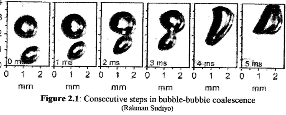
Firstly, the external flow governs whether the bubbles collide, the force of the collision and the contact time (Chesters, A. K., 1991). The consecutive steps in bubble coalescence can be explained within three steps as following (Oolman, T. O. and Blanch, H. W., 1986; Rahman Sudiyo);

a) Collision of bubbles

Two bubbles contact each other within the liquid phase.

b) Trapping and thinning of a thin liquid film

Upon collision impact, there is flattening of the bubbles surfaces in contact,

leaving a thin liquid film separating them. This film is typically 10"3 and 10"4 cm

in thickness. Coalescence will take place if the two bubbles stay in contact for longer than is required for the film to thin.

c) Film rupture

Once the film is sufficiently thin, an instability mechanism will result in film rupture and formation of a coalesced bubble. The entire process occurs on a millisecond time scale, the rate determining step being film drainage (Marrucci, G., 1969).

(14)

4 3

2

1 \

0 ^{2 ms}

0 1 2 0 1 2 0 1 2 0 1 2 0 1 2 0 1

mm mm mm mm mm mm

Figure 2.1: Consecutive steps in bubble-bubble coalescence

(Rahman Sudiyo)

m s

i — i — ' — r ^i—i—

Furthermore, whether the coalescence happens or not depends not only on the hydrodynamics and the surface properties but also on the external flow which governs the frequency, force and duration of the collisions (Tse et al., 1998). It is observed based on Figure 2.1 that the time required for two bubbles from the first contact to complete coalescence is about 2ms. The coalescence rate of bubbles is affected by two factors which are the frequency of collision and the probability that bubbles coalescence upon collision (Pilon et al., 2004). The first factor, frequency of collision in turn depends on

the liquid flow and on the hydrodynamics interactions between the bubbles and the

liquid phase.

Meanwhile the coalescence upon collision occurs when the collision duration

time, tc is larger than the time to drain the film between the bubbles, t± The probability of coalescence, P is expressed as a function of the collision duration time, tc and the

drainage time, td:

P = exp (-td/tc) (1)

In the limiting cases, the thinning of the film separating two colliding bubbles is dominated by either viscous or inertial forces. The Weber number, a dimensionless expression is generally used in the studies of bubble coalescence. This expression

represents the ratio of the inertial forces to the surface tension forces:

We = pV2r

(2)

(15)

Where, p denotes liquid density, V the relative velocity of centers of colliding bubbles, r the bubble radius and o the surface tension. Chesters (1991) has proposed an expression for each limiting cases by assuming that bubbles have the same radius and both gas viscosity and the van der Waals forces can be ignored:

—= (~-/ For inertia controlled drainage (Re°o <24) (3)

For viscosity controlled drainage (Reco > 24) (4)

3*1

-J2<rpr

Another introduced term jx in the above equation denotes liquid viscosity. For inertia controlled drainage, increasing in the superficial gas velocity will increase the average bubble velocity while the probability of coalescence upon collision decreases.

Otherwise, the probabilty of coalescence is independent of the superficial gas velocity.

In addition, the size of the resultant bubble is determined by the type of coalescence, which in turn depends on the tubes spacing and the instance of bubble expansion at which coalescence occurs (N.A. Kazakis et al., 2008).

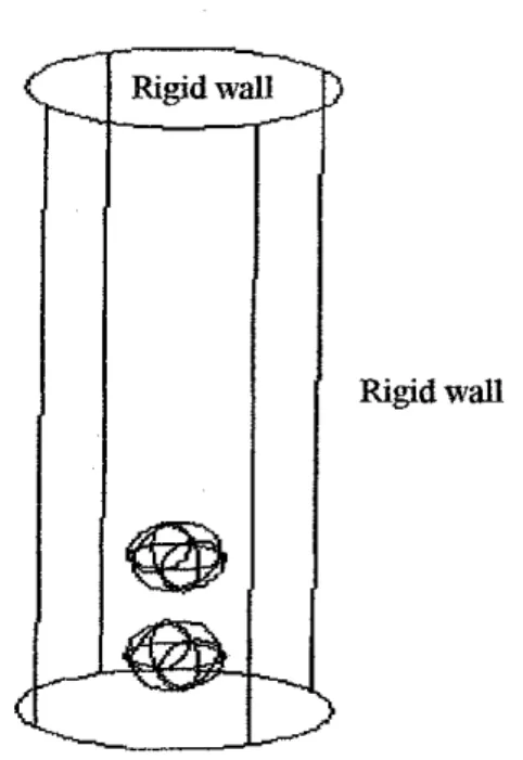
2.2 Bubble Transport

Rigid wall

Figure 2.2: Schematic diagram of co-axial bubbles (Li Chen et al., 1998)

(16)

From Li Chen et al. (1998), the motion of the two bubbles can be described by

the Navier-Stokes equation, which is written in a non-dimensional form as:

V • U = 0 (5)

dW + V-(pV ®ty^ -Vp +pg +±V •[M(VU + VVT)] + ±-Fsv (6)

3t \r -^ j r ra Re u~\ ja Bo

with scales:

p —-i:—i\j = ;x*=—-;t = ;

Pref "re/ «o *ref

p' = ^;„'=^-,a' = -^- (7)

Pref Ih-ef °ref V J

in which:

%ref —yd^Q'' Pref ~ Pref^ref- (p)

Note that * is omitted in equations (5) and (6) for convenience. ® denotes the inner product of tensors, U(urueuz) is the fluid velocity in x(r, 0,z), p the density, u, the dynamic viscosity, p the pressure, g(0,0,g) the gravity vector, Rq initial bubble radius, and Fsv the volume form of the surface tension force. The subscript, ref, stand for a reference value, and here, liquid properties are adopted as reference properties. Reynolds and Bond numbers are defined by:

and

Re=e2^.Bo =££££» (9)

ih-ef a v J

p(x, t) = F(x, t)pf + [1 - F(x, t)\ps;

p(x, t) = F(x,t)fif + [1 - F(x,t)]iig (10)

where i7 is the local volume fraction of one fluid. Its value may be unity in the liquid phase and zero in the gas phase if a gas-liquid two-phase system is involved. A value between 1 and 0 indicates a density interface. The last term of equation (6) is the surface tension force, which exists only at the interface and is modelled by the continuum surface tension force (CSF) method developed by Brackbill et al (1992). In this model, an interface is interpolated as a transient region with a finite thickness. Thus the surface tension force localised in this region can be converted into a volume force with the help

of a Dirac delta function concentrated on the surface. The surface tension force is written

as:

(17)

FSV =<TK(X)^ (11)

in which:

K - -(V • n) (12)

from the definition of a unit normal vector to a surface:

where c in the above equations is a colour function and [c] is the difference of the colour function between two phases.

It is noted that Equations (9) and (10) represent discontinuous properties of fluid, which imply an interface between two-phase fluids, and they can be used to monitor the dynamics of the interface. However, when a large discontinuity is involved, for example a discontinuity of 850 in density ratio exists for a water-air system, numerical difficulties may arise in identifying an 'exact' interface. Thus, instead of solving the density transport equation directly, the volume fraction of liquid, F, is used to identify an interface. The transport of the F function is governed by:

^+F-(UF) =0 (14)

Also, the colour function, where c, in Equations (11) and (13) can be replaced by F. Now suitable initial and boundary conditions are required. In the case studied in this paper, an initially spherical gas bubble is located on the axis of a vertical cylinder filled with a stationary liquid. The boundary conditions are U = 0 at the walls. The bubble is initially at rest.

2.3 Available Related Models

C.P. Ribeiro Jr and D. Mewes (2006) in their study have summarised the comparisons of models for film drainage that available in the literature which are in these models, the coalescence time is computed as the time required for the thin film of the continuous phase separating the interacting bubbles to drain from an initial thickness

to a critical value, at which film rupture, and hence coalescence, occurs. A summary of

the models available in the literature for pure liquids is given in Table 2.3.1.

(18)

Table 2.3.1: Available literature models for the coalescence time in pure liquids

(C.P. Ribeiro Jr., D. Mewes, 2006) Reference

Hodgson and Woods (1969)

Chesters and

Hofman(1982)

Chen etal (1984)

Oolman and

Blanch (1986)

Lee etal. (1987)

Jeelaniand Hartland (1994)

Li and Liu (1996)

Main assumptions Cylindrical drops; immobile interfaces; non-uniform film thickness; hydrostatic and inertia eifects neglected;

rupture at zero

thickness; van der Waals forces

included

Spherical bubbles; mobile interlaces; non-uniform film thickness; inviscid. gravity-free fluid; uniform velocity across the film; van der Waals forces neglected

Spherical bubbles; immobile interfaces; non-uniform film thickness; inertia effects neglected; analysis of the rate of thinning at the rim of the film; van der Waals forces included; linear stability analysis used to predict critical film thickness for rupture Spherical bubbles; mobile interfaces; plane-parallel film;

flat

velocity profile in the film; van der Waals forces included;

stagnant film at t - 0 Spherical bubbles; partially immobile interfaces; plane parallel

film; contributions of film thinning and rupture Spherical bubbles; mobile interfaces; newtonian liquid film with uniform thickness;

parabolic velocity profiles

inside the bubbles

Spherical bubbles; mobile interfaces: newtonian liquid

film with non-uniform

thickness; parabolic velocity profiles inside the bubbles; van

der Waals forces included

Relations

7/4

tc =

3tt 7}hrb

tc =

a

tr = 1.0704Wr/b[(pL-pG)gj3'5

CT6/5£2/5

d2S _1.5(d8\2 a2

2A

; «i - ; «2 = 3narR%

tc = min lA(/ic) + £2(/ic)]

tt(M = -3MrjLRi

r 8x3 |^ +

dx ^A 5 a - 2

t2(ftc) = 24n2Mar}Lh^A

t, = ZMlM

inch

a-fA2rb

6tcg2 4F/l21 +

o)J

1/7 K - 0.267

[rb (6jtx3)

- = 40.0£0-46 + 141.49/?0-26"102'a'

Sr]LRl

T — ;P

R%B

oh*^•; ^a

Vl

ZvcRd(Tb.i + n.,2)

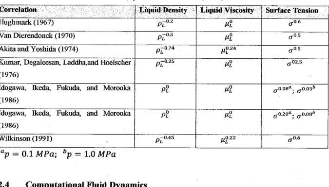
Meanwhile, Ryszard Pohorecki et al. (2001) has summarised the different correlations for the influence of liquid properties on the average bubble diameter as

shown in Table 2.3.2.

10

(19)

Table 2.3.2: Influence of liquid properties on the bubble diameter (Ryszard Pohorecki et al., 2001)

Correlation Liquid Density Liquid Viscosity Surface Tension

Hughmark(1967) Pl02 pl ^0-0-6

Van Dierendonck (1970) PZ03 P-l ^<r0-5

Akita and Yoshida (1974) PI074 ^0.24 _a05

Kumar, Degaleesan, Laddha,and Hoelscher (1976)

p-0.25

Pl ^a025

Idogawa, Ikeda, Fukuda, and Morooka (1986)

Pl f*l (JD.D8a. ^o.oa6

Idogawa, Ikeda, Fukuda, and Morooka (1986)

Pl Pl 0-0.20°. g.0.086

Wilkinson (1991) Pl0A5 ^0.22 ff0.6

ap = 0.1 MPa; bp = 1.0 MPa

2.4 Computational Fluid Dynamics

Computational fluid dynamics (CFD) is one of the branches of fluid mechanics that Uses numerical methods and algorithms to solve and analyze problems that involve fluid flows. CFD offers a qualitative prediction of fluid flows by means of mathematical modeling, numerical methods and software tools (Dmitri Kuzmin). Numerical solutions provided by CFD have allowed the analysis of complex phenomena without having to invest in complicated experimental measurement and expensive prototype (Fadlun, Verzicco et al., 2000). The most basic consideration in CFD is how to treat a continuous fluid in a discretized fashion on a computer. One of the methods is to discretize the spatial domain into small cells to form a volume mesh or grid. Next a suitable algorithm is applied to solve the equations of motion which either Euler equations for inviscid or Navier-Stokes equations for viscous flow.

At two-phase flow point of view, the modeling is still under development and different methods have been proposed in the flow analysis. Numerically, a robust algorithm with an accurate representation of interfaces is needed to handle the complex topological changes during the bubble fusion. In former literature, Volume-tracking

11

(20)

methods that account for the interface in an implicit way such as Volume-of-FIuid (VOF) or Level Set method are inprinciple suitable to represent the coalescence process.

Most of these methods are either good in maintaining a sharp interface or at conserving mass. This is important as the evaluation of the density, viscosity and surface tension in

based on the values averaged over the interface.

VOF method is commonly used as the numerical method for the dynamics and deformation for the liquid-air interface (J.M. Martinez et al.). In fact, this method is widely used for two phase flow simulations and shows a good agreement between numerical and experimental data. This technique is applied for tracking and locating the free surface or fluid-fluid interface. The VOF is an Eulerian fixed-grid technique and it belongs to the class of Eulerian methods which are characterized by a mesh whether is stationary or is moving in a certain prescribed manner to accommodate the evolving shape of the interface. Besides, the VOF method is known for its ability to conserve the mass of the traced fluid and also it can trace easily the topology changes by fluid

interface. In spite of this, a disadvantage on VOF method is the so-called artificial coalescence of gas bubbles which happens when their mutual distances is less than the

size of the computational cell (Deen, Annaland et al., 2009). Furthermore VOF model

however is inappropriate if bubbles are small compared to a control volume, namely

bubble column (Andre Bakker, 2002).

Recently, the nonstop development of computational power has been one on the driving force that encourages theusage of CFD for engineers. As forming a new trend in finding technological solutions, fluid dynamics simulations have raised some main

issues which are accuracy, computational efficiency and the ability to handle complex geometries. A real challenge in CFD comes when dealmg with complex fluid flow analysis. The simulation of a flow around a realistic configuration is extremely complex since the shape of the domain must include wetted surface of the geometry of interest (Iaccarino and Verzicco, 2003). Another factor that complicates the analysis when geometry complexity is combined with moving boundaries and high Reynolds numbers in which significantly increase the computational difficulties; since they require

12

(21)

regeneration or deformation of the grid and turbulence modelling (Fadlun, Verzicco et

al., 2000).

Looking for a recent advanced alternative in dealing with complex fluid flow analysis, the Immersed Boundary (IB) technique is introduced nowadays. This technique allows the solution of differential equations in complex geometric configurations on simple meshes by introducing forcing conditions on certain surfaces corresponding to the physical location of the complex boundaries (laccarino and Verzicco, 2003). This method is applied in such a way the bodies of almost arbitrary shape can be added without altering the computational grid, that considerably avoid a time-consuming

process (Yusof; 1998).

2.5 Volume-of-Fluid (VOF) Model

The VOF is formulated in principle that two or more phases are not interpreting.

In fact, for each additional phase added to the model, a variable is introduced which is

the volume fraction of the phase in the computational cell (Fluent Manual, 2003). In each control volume, the volume fractions of all phases sum to unity. As long the volume fraction of each phase is known at each location, the fields and properties are shared by phases and being represented as volume-averaged values. If the q-th fluid's volume fraction is denoted as a ctq hence three conditions are possible happened within a

cell:

a) Oq = 0; the cell is empty (of the q-th fluid) b) Oq = 1: the cell is full (ofthe q-th fluid)

c) 0< ctq <1; the cell contains the interface between the q-th fluid with one or

more others fluid

The tracking of the interface^) between the phases is generated by the solution of continuity equation for the volume fraction of one (or more) ofthephases.

dan . _, _ sa Pq

•a . -* w-r ^ " n

it+v-Va^-± 05)

13

(22)

The volume fraction equation will not be solved for the primary phase due to the

constraint as following:

Tq=Qaq = 1 (16)

The properties appearing in the transport equations are determined by the presence of the component phases in each control volume. Generally the volume- fraction-averaged density for an n-phase system can be expressed as equation 7. All other properties also take on the following form to be computed.

P = Z<*qPq

(17)

In VOF model, a single momentum equation used to solve throughout the domain and the resulting velocity is shared among the phases. The momentum equation is dependent on the volume fractions of all phases via the properties p and p. However shared-fields approximation has one limitation when a large velocity differences exist between the phases. The accuracy of the velocities computed near the interface can be

adversely affected. The momentum equation is shown below:

f (pv) +V. (p vv) =-Vp +V. [p(Vv +VvTy\ +pg+P (18)

The energy equation also shared among the phases and the VOF model treats

energy, E and temperature, T, as mass-averaged variables respectively shown below:

~ (pE) + V. (v(pE + p)) = V. (keffVT) 4- Sh (19)

b 2%=1«qpq <20>

In the above equation Eq for each phase is based on the specific heat of that phase and the shared temperature. The properties p and thermal conductivity, A^-are shared by the phases. Meanwhile the source term, Sh contains contributions from radiation, as well

as any other volumetric heat sources.

14

(23)

2.6 Modelling Case Overview

A case has been selected for modelling case which is taken from Li Chen et al.

(1998), entitled "The Coalescence ofBubbles - A Numerical Study". A literature review on the selected case is performed as below:

The team has studied the dynamics of bubble coalescence using a robust

numerical model for a multiphase flow system with interfaces. In their research, they

also investigated the effects of liquid viscosity and surface tension on bubble coalescence, for which Reynolds number ranges from 10 to 100 and Bond number ranges from 5 to 50.

In order to validate the numerical solution, Li Chen et al. (1998) had carried out

an experiment with a glycerin liquid with pf « 1220 kg/m3, \if = 0.11 kg/m.s, and

o = 0.006 N/m. The experimental procedure is taken from Manasseh et al. (1998)

where the air bubbles were produced from compressed and filtered air in pressure-

controlled mode. The underwater nozzle had internal diameter of 6.0 mm and it was

machined to maintain its internal edge as sharp as possible in ensuring a known contact radius of bubbles. The nozzle orifice was at depth of 0.23 m. The schematic diagram of

apparatus is shown from Figure 2.6.1.

Meanwhile, the equivalent radius of a spherical bubble was determined from the

acoustic frequency of bubble oscillation Manasseh (1997). These properties give

equivalent non-dimensional parameters which are Bo=5, M=4.1><10'3 and pf/pg&

1000 with a 10% error in both density and viscosity estimation. The similarity of the

bubble coalescence between the predicted and experimental results can be seen from Figures 2.6.2 and 2.6.3.

From both methods, the experimental result for the average rise velocity, with reference to the leading bubble centre before coalescence, gives 0.3ms"1, while the numerical simulation gives 0.24 ms"1. The validation gives an error of 20%. Based on

15

(24)

Figures 2.6.2 and 2.6.3, it is observed that the differences between the numerical and experimental following bubbles appear mostly in the first two frames. This happens due to the different initial conditions. However, the agreement between the results may be considered reasonable, given the somewhat different initialization and uncertain fluid properties in the experiment.

From the validation, it is shown that the numerical model used in this study can accurately capture the complex topological changes during the coalescence. The predicted behavior of bubble coalescence is in reasonable agreement with the experimental result. It is also found in this paper that with a high Reynolds number (low viscosity) a strong liquid jet formed behind the leading bubble inhibits the approach of the following bubble. Thus coalescence does not occur or is postponed. The effect of surface tension on bubble coalescence shows that; a lower surface tension results in an earlier coalescence because of severe stretching ofthe interface.

Strobe

Data-logger Triggering

circuit Oscilloscope

Amplifier

SLR camera

Hydrophone

Bandpass

filter

Valve

I

Figure 2.6.1: Schematic diagram of apparatus

(Manasseh etal., 1998)

16

s

Speaker

Pressure regulator

(25)

{a)x=i3

::::;:|S MM

:i::::^*T

will

I:

*Wj;: •

:;

(b) t=2.0 (e)x=23 (d)-C"3.G Figure 2.6.2: Predicted axisymmetric coalescence of two gas bubbles in a viscous liquid

(Re=12, Bo=5, M-4.1 xlO"3, pf/ pg=1000, u* /Ug=100, z/Ro=0.36)

(Li Chen et al., 1998)

(a) t=45 ms {b)t=60ms (c) t~75 rus {d)-E;=9Gim

Figure 2.6.3: Experimental observation ofthe axisymmetric coalescence of two gas bubbles in a glycerin liquid

(M=4.1*10-3, Bo=5, or/ pg~1000)

(Li Chen et al., 1998)

17

(26)

CHAPTER 3

METHODOLOGY / PROJECT WORK

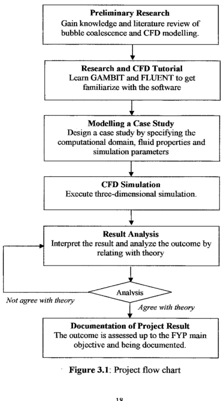
3.1 Project Flow Chart

Preliminary Research

Gain knowledge and hterature review of bubble coalescence and CFD modelling.

ir

Research and CFD Tutorial

Learn GAMBIT and FLUENT to get

familiarize with the software

i r

Modelling a Case Study Design a case study by specifying the computational domain, fluid properties and

simulation parameters

ir

CFD Simulation

Execute three-dimensional simulation.

1f

Result Analysis

Interpret the result and analyze the outcome by relating with theory

<!! Analysis J>- Not agree with theory

Agree with theory

Documentation of Project Result The outcome is assessed up to the FYP main

objective and being documented.

Figure 3.1: Project flow chart

18

(27)

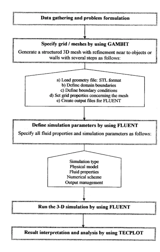
3.2 Project Work Execution

Data gathering and problem formulation

Specify grid / meshes by using GAMBIT

Generate a structured 3D mesh with refinement near to objects or walls with several steps as follows:

a) Load geometry file: STL format b) Define domain boundaries c) Define boundary conditions d) Set grid properties concerning the mesh

e) Create output files for FLUENT

Define simulation parameters by using FLUENT Specify all fluid properties and simulation parameters as follows:

Simulation type Physical model Fluid properties

Numerical scheme

Output management

™«S^5HiUia^S5ES3ES?»!^&Ji;

Run the 3-D simulation by using FLUENT

Result interpretation and analysis by using TECPLOT

Figure 3.2: Project work execution

19

(28)

3.3 Proj ect Gantt Chart

?nW"- Detail/Week 1 2 3 4 5 6 7 8 9 10 i t 12 13 14 i Selection of project topic

2 Preliminary research

3 Submission of preliminary

report m

4 Project work starts -.-":

5 Submission of progress

report m>

6 Seminar m

7 Project work continues

8 Submission of interim report _m

9 Oral presentation _m

Figure 3.3.1: Gantt chart of FYP 1

:JS6.;- Detail/ Week 1 2 3 4;. 5 6 7 8 9 10 i i 12 13 14 15 16 17 18 19

1 Project work continues . - - - _ ,

-•;•- ^:.::-.

2 Submission of progress

report 1 ^m>

3 Project work continues ^-

4 Submission ofprogress

report 2 ^—- m

5 Project work continues

6 Poster exhibition

m

7 Submission of dissertation

report (soft bound) ®

8 Oral presentation _®

9 Submission of dissertation

report (hard bound) ^m

Figure 3.3.2: Gantt chart of FYP 2

Le^nd: ® Milestone Activities

20

(29)

3.4 Tools and Equipment

The main tool required in this Bubble-Bubble Coalescence Project is Computational Fluid Dynamics software. The simulation is handled with a systematic procedure shown in Figure 3.2. However for all CFD software, a basic procedure applied. Briefly, during pre-processing, the geometry of the problem is first defined.

The volume occupied by the fluid is then divided into mesh. After that, the physical modelling, boundary conditions and fluid properties are further specified. The simulation is started and the equations are solved iteratively. Lastly the result is analyzed by using a

processor.

In this project, the simulation will use FLUENT as the software to study the dynamics of coalescence phenomenon. GAMBIT is used to draw and mesh the 3-D computational domain for the problem. The simulation will be done to study the behaviour of bubble coalescence and effect of certain model parameters on the bubble properties. Other tools used are TECPLOT for post-processing and AutoCAD for technical drawing purpose.

21

(30)

CHAPTER 4

RESULTS AND DISCUSSION

4.1 The Behavior of Bubble Coalescence

4.1.1 Modelling

In modelling the framework, several assumptions have been specified to the system (as stated in the scope of study):

• Laminar and low Reynolds number of flow

• Liquid and gas are isothermal and incompressible

• Two co-axial bubbles with the identical radius rising in line

• Bubble is free rising under gravity presence

• Cylindrical tank is used

The fluid selected into this case is water (liquid) and oil (bubbles). With these

fluid properties of water-oil system, calculation had been done in order to obtain some value of parameters, namely bubble radius, and velocity of the bubbles.

a) Bubble radius, n,

In this modelling, the bubble radius is calculated by using the correlation given

by Minnaert (1933). Minnaert (1933) has found the fundamental relation between bubble

acoustic frequency and radius by equating the potential energy of the compressed gas at

one node of the oscillation cycle, with the kinetic energy of the fluid set in motion

around the bubble at the antinode:

^=m <*>

where the values are:

/ —frequency

22

(31)

/ = 0.95 ± 0.002 kHz = 950/s

-> acoustic frequency from the first period of oscillation, Manasseh (1998)

Pf = liquid density pf = 997 kg/m3

Pn = absolute liquid pressure Po = Patm + Pf9h

1.01325 xlO5 kg^

Pn =

P0 = 103574.5 kg/ms2

v = ratio of specify heats for the gas (air}

y = 1.401

-> at temperature 20°C, refer APPENDIX A.

substituting the values into equation (21):

f\ (997 kg\ /9.81m\

/950\

H~)=

3(1.401) C

103574.5 kg

ms2

(997_kg\ 2

^ Xm3 )r*

rb = 0.0031723 m = 0.00317 m = 3.17 mm.

From Manasseh et al. (1998) study, the larger bubbles of 2-4 mm radius were

examine since these are of greater industrial relevance and also permits closer

visualisation of the bubble dynamics. Meanwhile, the bubble radius obtained from the

calculation is 3.17 mm which lies in the range between 2-4 mm of radius, thus the value

is considered to be reasonable.

b) Velocity of bubble, v*

The velocity of the bubble can be estimated from equation (22):

vb =W^ (22)

where other values are:

23

(32)

a = gravity

g - 9.81 m/s2 Pf = viscosity

pf = 1.04 x 10-3 kg/ms

@(0.00317^(g^)(g^H)

/1.04 x 10~3 kg"

vb =21.001 m/s

vb -

m s

cl Initial distance between successive bubbles. S

An assumption has been done in order to specify the spacing between the bubbles as following:

S = 3rb (23)

substituting the obtained value of rb into equation (23):

S = 3(3.17 mm) = 9.51 mm

Note that D is the distance from the bubble centre to another bubble centre.

Figure 4.1.1: Computational domain

24

(33)

The boundary conditions and the relevant parameters ofthe case study have been

tabulated in Table 4.1.

Table 4.1: Boundary conditions and fluid properties

Grid / boundary conditions

Tank domain Cylinder with r=10 mm, fr=60 mm Boundary conditions All boundaries are wall.

Refinement method Refine blocks

Spacing 9.51 mm (spacing between bubbles centre)

Bubble size Two bubbles with radius of 3.17 mm

Bubble location Two bubbles are aligned in the centre of the cylindrical domain with different height:

hr=5.17mm h2= 14.68 mm

Fluid properties / simulation parameters

Simulation parameters

Simulation model Volume-of-Fluid (VOF) Simulation type Unsteady, implicit

Fluid

properties

Phase 1 (Bubbles) Oil

Density

800 kg/m3

Viscosity 0.00168 kg/m.s

Phase 2 (Liquid) Water

Density

997 kg/m3

Viscosity

1.04 x 10"3kg/m.s

Surface tension 0.023 N/m

Operating

conditions

Operating pressure 101.325 kPa

Operating density

800 kg/m3 (density of oil)

Gravity acceleration 9.81 m/s2

25

(34)

4.1.2 Result and Discussion

a) t = 0.32 s b) t = 0.33 s

c) t = 0.34 s d)t-0.35 s

Figure 4.1.2: Series of contours ofvolume fraction

Figure 4.1.2 shows the some relevant plots of contours of volume fraction during

bubble coalescence process of two bubbles. The behaviour of bubble coalescence is

investigated. At initial condition t = 0s, the two spherical bubbles were stationary and when simulation began, the bubbles were observed to start rising due to the buoyancy force. As time progresses, the two spherical bubbles became ellipsoids in shape due to pressure difference between thetop and bottom surfaces of the bubbles. Based on Figure 4.1.2 a, the liquid circulation around the bubble produced a jet to push in the lower

surface of both leading and following bubbles and the deformations of the bubbles occur. The pressure, behind the leading bubble controlled the entrainment of the

following bubble by promoting a slight acceleration and elongation of the following bubble which eventually causes the coalescence to occur(Li Chen et al., 1998).

As thebubbles started approaching each other at t = 0.34 ms (Figure 4.1.2 c), the following bubbles accelerates and then collided. Upon collision impact, there is

26

(35)

flattening of the bubbles surfaces in contact, leaving a thin liquid film separating them (Figure 4.1.2 d). Coalescence will take place if the two bubbles stay in contactfor longer than is required for the film to thin (Oolman, T. O. and Blanch, H. W., 1986). Once the film is sufficiently thin, an instability mechanism will result in film rupture and

formation of a coalesced bubble.

100 150 200 250

Time (ms)

300

Figure 4.1.3: Position oftwo bubbles as a function of time

The bubble trajectories are plotted as shown in Figure 4.1.3. Based on the figure,

it is observed that the bubbles which are top and the bottom bubbles start to rise and approach each other as the time progresses. The distance between the two bubbles is getting smaller until it coalesced estimated at t = 0.35 s.

27

(36)

4.2 The Effect of Surface Tension on Bubble Coalescence

4.2.1 Modelling

A case has been selected for validation which istaken from Li Chen et al. (1998), entitled "The Coalescence of Bubbles - A Numerical Study". The literature review on the selected case can be referred to previous Section 2.6.To start modelling, the bubble radius is calculated from the parameters given. In the validation, the values of time is

represented in dimensionless time, t. Thus we also need to calculate the value of

reference time, tTef in our calculation in order to obtain the real time values, treal. The

related calculations are shown as below:

Given the parameters as follows:

pf = 1220 kg/m3

pf = 1.7894 x 10"3 kg/m.s a = 0.066 N/m = 0.066 kg/s2

Re = 10 Bo = 5

as the relative ratio of density and viscosity are given by:

Pf/pg=850and Uf/Ug=100

therefore:

pg = 1.435 kg/m3

pg = 1.7894 x lO"5 kg/m.s

al Bubble radius. Rh

In this modelling, the bubble radius is calculated by using the dimensionless

correlation as follows:

Reynolds number = Re=^ = R^R^°^f (24)

28

(37)

0.5 /•?.OI 77Z.1

//r /1.7894

m/s fl& = 2.799 x 10"4 m

, ,„, (9.81 m}05 /1220 kg\ 15

_Rb(gRby-5Pf ^K^2^) { m3 )Rb

Pf (1.7894xl0~3 kg}

bl Relative velocity, u^^

Relative velocity can be computed from this formula as follows:

Urel = 49^b (25)

Urel

Urel = 0.0524 m/s

cl Reference time, tVOf

Reference time can be computed from this formula as follows:

W =^ (26)

/9.81m\

= ( —J (2.799 x 10"4 m)

_ 2.799 x 10~4 m re/ 0.0524 m/s

tref = 5.342 x 10~3 s = 5.342 ms

d) Real time, tron,

The dimensionless time is given by this formula:

treal tref

T=tXeal (2?)

For example of calculation, real time, treal at dimensionless time of t^0.5 can be computed as follow:

treal = t x tref = 0.5 X (5.342 x 10~3 s) = 2.671 X 10"3 s

29

(38)

Thevalues of tj.eal are computed for several values of x ranging from 0.5 to 3 as

shown in table below. The position of two bubble centres as a function of time will be read at treal from the simulation.

Table 4.2.1: Real time data

T 0.5 1.0 1.5 2.0 2.5 3.0

tn-al(s) 0.002671 0.005342 0.008013 0.010684 0.013355 0.016026

e> Tank dimension

The tank used is cylindrical with the dimension is assumed as follows:

Tankradius = Rt = 10Rb

(28)

Tank height = Ht = 40Rb (29)

substituting the obtained value of Rb into equation (28) and (29):

Rt = 10(2.799 x 10~4 m) = 2.799 x 10~3 m Ht = 40(2.799 x 10~4 m) = 0.011196 m

ft Initial distance between successive bubbles. -V

An assumption has beendonein orderto specify the spacing between the bubbles

as following:

S = 2.36i?6 (30)

substituting the obtained value of Rb into equation(30):

5 = 2.36(2.799 x 10~4 m) = 6.606 x 10"4 m

where S is the distance from the bubble centre to another bubble centre.

g) Bubbles location

Two bubbles are initially aligned in the centre of the cylindrical tank with different height, hi for bottom (following) bubble and h2 for top (leading) bubble:

hi = 4Rb (31)

30

(39)

h2 = h±+S (32) substituting the values into equation (31) and (32):

^ = 4(2.799 x 10"4 m) = 1.1196 x 10"3 m

h2 = (1.1196 x 1G"3 m) + (6.606 x 10"4 m) = 1.7802 x 10"3 m

where hi and h2 are measured from the tank bottom to the each bubble centre respectively. The data calculated are tabulated in Table 4.2.2. The sketch and illustration of computational domain with the specified dimension is shown in Figure 4.2.1.

Table 4.2.2: Boundary conditions and fluid properties Grid / boundary conditions

Tank domain Cylinder with Rt = 2.799 x 10"3 m, Ht = 0.011196 m Boundary conditions All boundaries are wall.

Refinement method Refine blocks

Spacing, S

6.606 x 10-4 m (spacing between bubbles centre)

Bubble radius, Rb 2.799 x 10"4 m

Bubble location h^ 1.1196 x 10"3 m, h2= 1.7802 x 10"3 m Fluid properties / simulation parameters

Simulation parameters

Simulation model Volume-of-Fluid (VOF) Simulation type Unsteady, implicit

Fluid

properties

Phase 1

(Bubbles)

Density, pg 1.435 kg/m3

Viscosity, Ug 1.7894 xl0-s kg/m.s

Phase 2

(Liquid)

Density, pf 1220 kg/m3

Viscosity, Uf 1.7894 xl0~3 kg/m.s Surface tension, o 0.066 N/m = 0.066 kg/s2 Operating

conditions

Operating pressure 101.325 kPa

Operating density 1.435 kg/m3 (density of bubbles) Gravity acceleration 9.81 m/s2

31

(40)

(0,0.011196)

(0, 1.7802x10°)

S = 2.36R,,

(0, 1.1196X10"3)*

4R,,

(0, 0) * fc. (2.799x10 3, 0) Rt = 10R,, =2.799xl0^m

I.4E-02

Computational Domain &.

Initial Bubble Location

I.2E-Q3

I.DE-02

J.0&03-

i.OE-03

-

I.OE-03

i.OE-03

.0E*OO

< )

o.oooe+oo

Y

(2.799xl0"35 0.011196)

Ht = 40Rb=0.011196m

Mesh between the Bubbles

Mesh Inside a Bubble

Figure 4.2.1: Computational domain

32

(41)

By using constant parameter of bubble radius, Rb = 2.799 x 10~4 m, another two test cases also be performed to study the effect of surface tension on bubble coalescence. The original case (Case 1) and other 2 cases' parameters have been tabulated at different values of Re and Bo number as shown in Table 4.2.3. The Re and Bo are changed by manipulating the value of hquid density and surface tension

respectively; while other values like viscosities, density ratio and viscosity ratio are kept

constant.

Table 4.2.3: Parameters for simulation test cases Test

Case

1

Reynolds

number

(Re)

Bond number

(Bo)

Density

ratio

(Pf/Pa)

Viscosity

ratio

(|ii/h)

10 5 850 100

2 10 50 850 100

3 8.5 4.25 850 100

4.2.2 Result and Discussion

x=2.0

\C / \C

t=25 t=3.0

Figure 4.2.2: Predicted axisymmetric coalescence (Case 1) (Re=10, Bo=5, pf/ Pg-850, u.f /ug-100)

(Li Chen etal, 1998)

33

^3.5

(42)

a) x = 2.0

£b>

a) t - 2.0 (t-0.010684 s)

b)x = 2.5

£ ^

b)x = 2.5 (t = 0.013355 s)

c)r-3.0 d)x-3.5

c)t = 3.0 (t = 0.016026 s) Figure 4.2.3: Simulated axisymmetric coalescence (Case 1)

(Re-10, Bo-5, pf/ pg=850, jjf7^=100)

Both Figure 4.2.2 and 4.23 show a part of contours of volume fraction series for development of bubble coalescence at Re=10 and Bcf^5. The changes in the bubbles shape are carefully observed. The result obtained from CFD simulation (Figure 4.2.3) is compared with the predicted result from Li Chen et.al, 1998 (Figure 4.2.2). The outcome shows both results are closely agree with each other.

34

(43)

Based on the simulation result (Figure 4.2.3), the bubbles starts closely approaching each other at x^2. At this point, a pear-like shape is observed for the bottom (following) bubble. This happens due to the hquid jet behind the leading bubble which induces a severe deformation of the following bubble. The impact of the following bubble has terminates the vortex around the leading bubble, resulting a big circulation around those bubbles as a whole is gradually formed. Therefore, the liquid jet behind the leading bubble may be slightly smeared resulting in a spherical-cap-shaped leading bubble (Figure 4.2.3 a).

Meanwhile upon the collision, significant touch between those two bubbles then gives a mushroom-like shape in observation (Figure 4.2.3 c). When the two bubbles are in contact, because the surface tension always acts as a force reducing surface energy, the lower surface of the coalesced bubble is accelerated and a larger spherical cap is obtained (Figure 4.2.3 d).

The mechanism on bubble coalescence has been briefly explained in previous Section 4.1.2. Note that there is a distinct difference in shape changes between the results obtained in Figure 4.1.2 and the new result obtained in this section. As referring back to Figure 4.12, the two spherical bubbles became slightly ellipsoids in shape due to pressure difference between the top and bottom surfaces of the bubbles as the time progresses. However in the new result as shown in Figure 4.2.3, both bubbles change significantly in shape when coalesce. It is observed that this phenomenon happens because of the significant difference in the selection values of density ratio between those two simulations. The simulation result from Figure 4.12 is having pf / pg =1.25, while we are having pf/ pg=850 for simulation indicated in Figure 4.2.3. Thus, it can be concluded that the density difference between gas and liquid may affect the behaviour of bubble coalescence in terms of mechanism (shape changes). Higher density ratio shows vigorous changes in shapes that may be caused by higher resultant liquid jet (pressure) between top and bottom of the bubbles.

35

(44)

71 4^ ^{^TT} ^

/"*'•v" rfc^ Z 7

^ 1^-.

x=1.0 T=1.5 t=2j x=25

Figure 4.2.4: Predicted axisymmetric coalescence (Case 2) (Re=10, Bo=50, pf/ pg=850, pf /ug-100)

(Li Chen etal., 1998)

a)x=1.0 b)t=L5 b)x = 2.0

cb

b) x = 2.5

Figure 4.2.5: Simulated axisymmetric coalescence (Case 2) (Re=10, Bo-50, pf/ pg=850, u* 7^=100)

For further validation, the simulation for Re=10 and Bo=50 also has been performed. The shapes changes and coalescence time can be observed. The result