Smooth Manifolds and Observables
123
S. Axler F.W. Gehring K.A. Ribet
Mathematics Department Mathematics Department Mathematics Department
San Francisco State East Hall University of California,
University University of Michigan Berekeley
San Francisco, CA 94132 Ann Arbor, MI 48109 Berkeley, CA 94720-3840
USA USA USA
[email protected] [email protected] [email protected]
Library of Congress Cataloging-in-Publication Data Nestruev, Jet.
Smooth manifolds and observables / Jet Nestruev.
p. cm.—(Graduate texts in mathematics ; 220) Includes bibliographical references and index.
ISBN 0-387-95543-7 (alk. paper)
1. Manifolds (Mathematics) I. Title. II. Series.
QA613 .N48 2002
516'.07—dc21 2002026664
ISBN 0-387-95543-7 Printed on acid-free paper.
© 2003 Springer-Verlag New York, Inc.
All rights reserved. This work may not be translated or copied in whole or in part without the written permission of the publisher (Springer-Verlag New York, Inc., 175 Fifth Avenue, New York, NY 10010, USA), except for brief excerpts in connection with reviews or scholarly analysis. Use in con- nection with any form of information storage and retrieval, electronic adaptation, computer software, or by similar or dissimilar methodology now known or hereafter developed is forbidden.
The use in this publication of trade names, trademarks, service marks, and similar terms, even if they are not identified as such, is not to be taken as an expression of opinion as to whether or not they are subject to proprietary rights.
Printed in the United States of America.
9 8 7 6 5 4 3 2 1 SPIN 10885698
Typesetting: Pages created by the authors using a Springer TeX macro package.
www.springer-ny.com
Springer-Verlag New York Berlin Heidelberg
A member of BertelsmannSpringer Science+Business Media GmbH Mathematics Subject Classification (2000): 58-01, 58Jxx, 55R05, 13Nxx, 8
Preface to the English Edition
The author is very pleased that his book, first published in Russian in 2000 by MCCME Publishers, is now appearing in English under the auspices of such a truly classical publishing house as Springer-Verlag.
In this edition several pertinent remarks by the referees (to whom the author expresses his gratitude) were taken into account, and new exercises were added (mostly) to the first half of the book, thus achieving a better balance with the second half. Besides, some typos and minor errors, noticed in the Russian edition, were corrected. We are extremely grateful to all our readers who assisted us in this tiresome bug hunt. We are especially grateful to A. De Paris, I. S. Krasil’schik, and A. M. Verbovetski, who demonstrated their acute eyesight, truly ofdegli Lincei standards.
The English translation was carried out by A. B. Sossinsky (Chapters 1–8), I. S. Krasil’schik (Chapter 9), and S. V. Duzhin (Chapters 10–11) and reduced to a common denominator by the first of them; A. M. Astashov prepared new versions of the figures; all the TEX-nical work was done by M. M. Vinogradov.
In the process of preparing this edition, the author was supported by the Istituto Nazionale di Fisica Nucleare and the Istituto Italiano per gli Studi Filosofici. It is only thanks to these institutions, and to the efficient help of Springer-Verlag, that the process successfully came to its end in such a short period of time.
Jet Nestruev Moscow–Salerno April 2002
Preface
The limits of my language are the limits of my world.
— L. Wittgenstein This book is a self-contained introduction to smooth manifolds, fiber spaces, and differential operators on them, accessible to graduate students special- izing in mathematics and physics, but also intended for readers who are already familiar with the subject. Since there are many excellent textbooks in manifold theory, the first question that should be answered is, Why another book on manifolds?
The main reason is that the good old differential calculus is actually a particular case of a much more general construction, which may be de- scribed as the differential calculus over commutative algebras. And this calculus, in its entirety, is just the consequence of properties of arithmeti- cal operations. This fact, remarkable in itself, has numerous applications, ranging from delicate questions of algebraic geometry to the theory of ele- mentary particles. Our book explains in detail why the differential calculus on manifolds is simply an aspect of commutative algebra.
In the standard approach to smooth manifold theory, the subject is de- veloped along the following lines. First one defines the notion of smooth manifold, say M. Then one defines the algebraFM of smooth functions onM, and so on. In this book this sequence is reversed: We begin with a certain commutativeR-algebra1F, and then define the manifoldM=MF
1Here and belowRstands for the real number field. Nevertheless, and this is very important, nothing prevents us from replacing it by an arbitrary field (or even a ring) if this is appropriate for the problem under consideration.
as theR-spectrum of this algebra. (Of course, in order thatMFdeserve the title of a smooth manifold, the algebraF must satisfy certain conditions;
these conditions appear in Chapter 3, where the main definitions mentioned here are presented in detail.)
This approach is by no means new: It is used, say, in algebraic geometry.
One of its advantages is that from the outset it is not related to the choice of a specific coordinate system, so that (in contrast to the standard analytical approach) there is no need to constantly check that various notions or properties are independent of this choice. This explains the popularity of this viewpoint among mathematicians attracted by sophisticated algebra, but its level of abstraction discourages the more pragmatically inclined applied mathematicians and physicists.
But what is really new in this book is the motivation of the algebraic approach to smooth manifolds. It is based on the fundamental notion of observable, which comes from physics. It is this notion that creates an intuitively clear environment for the introduction of the main definitions and constructions. The concepts ofstate of a physical systemandmeasuring deviceendow the very abstract notions ofpoint of the spectrumandelement of the algebraFM with very tangible physical meanings.
One of the fundamental principles of contemporary physics asserts that what exists is only that which can be observed.In mathematics, which is not an experimental science, the notion of observability was never considered seriously. And so the discussion of anyexistence problemin the formalized framework of mathematics has nothing to do with reality. A present-day mathematician studies sets supplied with various structures without ever specifying (distinguishing) individual elements of those sets. Thus their observability, which requires some means of observation, lies beyond the limits of formal mathematics.
This state of affairs cannot satisfy the working mathematician, especially one who, like Archimedes or Newton, regards his science as natural philos- ophy. Now, physicists, for example, in their study of quantum phenomena, come to the conclusion that it is impossible in principle to completely distinguish the observer from the observed. Hence any adequate mathe- matical description of quantum physics must include, as an inherent part, an appropriate formalization of observability.
Scientific observation relies on measuring devices, and in order to intro- duce them into mathematics, it is natural to begin with its classical parts, i.e., those coming from classical physics. Thus we begin with a detailed ex- planation of why the classical measuring procedure can be translated into mathematics as follows:
Physics lab −→ Commutative unital R-algebraA
Measuring device −→ Element of the algebraA State of the observed −→ Homomorphism of unital physical system R-algebrash:A→R Output of the measu- −→ Value of this functionh(a),
ring device a∈A
In the framework of this approach, smooth (i.e., differentiable) man- ifolds appear as R-spectra of a certain class of R-algebras (the latter are therefore calledsmooth), and their elements turn out to be the smooth func- tions defined on the corresponding spectra. Here theR-spectrum of some R-algebraA is the set of all its unital homomorphisms into theR-algebra R, i.e., the set that is “visible” by means of this algebra. Thus smooth manifolds are “worlds” whose observation can be carried out by means of smooth algebras. Because of the algebraic universality of the approach de- scribed above, “nonsmooth” algebras will allow us to observe “nonsmooth worlds” and study their singularities by using the differential calculus. But this differential calculus is not the naive calculus studied in introductory (or even “advanced”) university courses; it is a much more sophisticated construction.
It is to the foundations of this calculus that the second part of this book is devoted. In Chapter 9 we “discover” the notion of differential operator over a commutative algebraand carefully analyze the main notion of the classical differential calculus, that of the derivative (or more precisely, that of the tangent vector). Moreover, in this chapter we deal with the other simplest constructions of the differential calculus from the new point of view, e.g., with tangent and cotangent bundles, as well as jet bundles. The latter are used to prove the equivalence of the algebraic and the standard analytic definitions of differential operators for the case in which the basic algebra is the algebra of smooth functions on a smooth manifold. As an illustration of the possibilities of this “algebraic differential calculus,” at the end of Chapter 9 we present the construction of the Hamiltonian formalism over an arbitrary commutative algebra.
In Chapters 10 and 11 we study fiber bundles and vector bundles from the algebraic point of view. In particular, we establish the equivalence of the category of vector bundles over a manifold M and the category of finitely generated projective modules over the algebraC∞(M). Chapter 11 is concluded by a study of jet modules of an arbitrary vector bundle and an explanation of the universal role played by these modules in the theory of differential operators.
Thus the last three chapters acquaint the reader with some of the sim- plest and most thoroughly elaborated parts of the new approach to the differential calculus, whose complete logical structure is yet to be deter-
mined. In fact, one of the main goals of this book is to show that the discovery of the differential calculus by Newton and Leibniz is quite simi- lar to the discovery of the New World by Columbus. The reader is invited to continue the expedition into the internal areas of this beautiful new world, differential calculus.
Looking ahead beyond the (classical) framework of this book, let us note that the mechanism ofquantum observabilityis in principle of cohomologi- cal nature and is an appropriate specification of those natural observation methods of solutions to (nonlinear) partial differential equations that have appeared in thesecondary differential calculusand in the fairly new branch of mathematical physics known ascohomological physics.
The prerequisites for reading this book are not very extensive: a stan- dard advanced calculus course and courses in linear algebra and algebraic structures. So as not to deviate from the main lines of our exposition, we use certain standard elementary facts without providing their proofs, namely, partition of unity, Whitney’s immersion theorem, and the theorems on implicit and inverse functions.
* * *
In 1969 Alexandre Vinogradov, one of the authors of this book, started a seminar aimed at understanding the mathematics underlying quantum field theory. Its participants were his mathematics students, and several young physicists, the most assiduous of whom were Dmitry Popov, Vladimir Kholopov, and Vladimir Andreev. In a couple of years it became apparent that the difficulties of quantum field theory come from the fact that physi- cists express their ideas in an inadequate language, and that an adequate language simply does not exist (see the quotation preceding the Preface).
If we analyze, for example, what physicists call the covariance principle, it becomes clear that its elaboration requires a correct definition of differ- ential operators, differential equations, and, say, second-order differential forms.
For this reason in 1971 a mathematical seminar split out from the phys- ical one, and began studying the structure of the differential calculus and searching for an analogue of algebraic geometry for systems of (nonlin- ear) partial differential equations. At the same time, the above-mentioned author began systematically lecturing on the subject.
At first, the participants of the seminar and the listeners of the lectures had to manage with some very schematic summaries of the lectures and their own lecture notes. But after ten years or so, it became obvious that all these materials should be systematically written down and edited. Thus Jet Nestruev was born, and he began writing an infinite series of books entitled Elements of the Differential Calculus. Detailed contents of the first install- ments of the series appeared, and the first one was written. It contained, basically, the first eight chapters of the present book.
Then, after an interruption of nearly fifteen years, due to a series of objective and subjective circumstances, work on the project was resumed, and the second installment was written. Amalgamated with the first one, it constitutes the present book. This book is a self-contained work, and we have consciously made it independent of the rest of the Nestruev project. In it the reader will find, in particular, the definition of differential operators on a manifold. However, Jet Nestruev has not lost the hope to explain, in the not too distant future, what a system of partial differential equations is, what a second-order form is, and some other things as well. The reader who wishes to have a look ahead without delay can consult the references appearing on page 217. A more complete bibliography can be found in [8].
Unlike a well-known French general, Jet Nestruev is a civilian and his personality is not veiled in military secrecy. So it is no secret that this book was written by A. M. Astashov, A. B. Bocharov, S. V. Duzhin, A. B. Sossin- sky, A. M. Vinogradov, and M. M. Vinogradov. Its conception and its main original observations are due to A. M. Vinogradov. The figures were drawn by A. M. Astashov. It is a pleasure for Jet Nestruev to acknowledge the role of I. S. Krasil’schik, who carefully read the whole text of the book and made several very useful remarks, which were taken into account in the final version.
During the final stages, Jet Nestruev was considerably supported by Is- tituto Italiano per gli Studi Filosofici (Naples),Istituto Nazionale di Fisica Nucleare (Italy), and INTAS (grant 96-0793).
Jet Nestruev Moscow–Pereslavl-Zalesski–Salerno April 2000
Contents
Preface to the English Edition v
Preface vii
1 Introduction 1
2 Cutoff and Other Special Smooth Functions on Rn 13
3 Algebras and Points 21
4 Smooth Manifolds (Algebraic Definition) 37
5 Charts and Atlases 53
6 Smooth Maps 65
7 Equivalence of Coordinate and Algebraic Definitions 77
8 Spectra and Ghosts 85
9 The Differential Calculus
as a Part of Commutative Algebra 95
10 Smooth Bundles 143
11 Vector Bundles and Projective Modules 161
Afterword 207 Appendix
A. M. Vinogradov Observability Principle, Set Theory and
the “Foundations of Mathematics” 209
References 217
Index 219
1
Introduction
1.0. This chapter is a preliminary discussion offinite-dimensional smooth (infinitely differentiable)real manifolds, the main protagonists of this book.
Why are smooth manifolds important?
Well, we livein a manifold (a four-dimensional one, according to Ein- stein) and on a manifold (the Earth’s surface, whose model is the sphere S2). We are surrounded by manifolds: The surface of a coffee cup is a man- ifold (namely, the torusS1×S1, more often described as the surface of a doughnut or an anchor ring, or as the tube of an automobile tire); a shirt is a two-dimensional manifold with boundary.
Processes taking place in nature are often adequately modeled by points moving on a manifold, especially if they involve no discontinuities or catas- trophes. (Incidentally, catastrophes — in nature or on the stock market — as studied in “catastrophe theory” may not be manifolds, but then they are smooth maps of manifolds.)
What is more important from the point of view of this book, is that manifolds arise quite naturally in various branches of mathematics (inal- gebra andanalysis as well as ingeometry)and its applications (especially mechanics). Before trying to explain what smooth manifolds are, we give some examples.
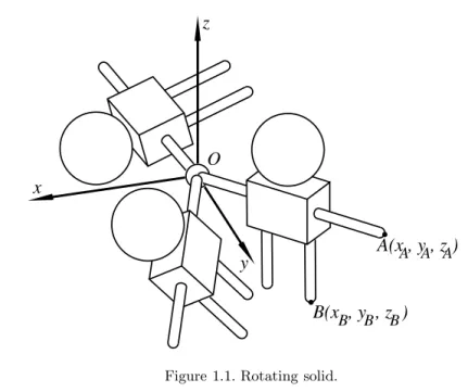
1.1. The configuration space Rot(3) of a rotating solid in space.
Consider a solid body in space fixed by a hingeO that allows it to rotate in any direction (Figure 1.1). We want to describe the set of positions of the body, or, as it is called in classical mechanics, its configuration space.
One way of going about it is to choose a coordinate system Oxyz and
O x
y z
A(x , y , z )
B(x , y , z )
A A A
B B B
Figure 1.1. Rotating solid.
determine the body’s position by the coordinates (xA, yA, zA), (xB, yB, zB) of two of its pointsA, B. But this is obviously not an economical choice of parameters: It is intuitively clear that only three real parameters are required, at least when the solid is not displaced too greatly from its initial position OA0B0. Indeed, two parameters determine the direction of OA (e.g., xA, yA; see Figure 1.1), and one more is needed to show how the solid is turned about theOAaxis (e.g., the angleϕB =B0OB, whereAB0 is parallel toA0B0).
It should be noted that these are not ordinary Euclidean coordinates; the positions of the solid do not correspond bijectively in any natural way to ordinary three-dimensional spaceR3. Indeed, if we rotateAB through the angleϕ= 2π, the solid does not acquire a new position; it returns to the positionOAB; besides,twopositions ofOAcorrespond to the coordinates (xA, yA): For the second one,Ais below theOxy plane. However,locally, say near the initial position OA0B0, there is a bijective correspondence between the position of the solid and a neighborhood of the origin in 3- spaceR3, given by the mapOAB→(xA, yA, ϕB). Thus the configuration space Rot(3) of a rotating solid is an object that can be described locally by three Euclidean coordinates, butgloballyhas a more complicated structure.
1.2. An algebraic surface V. In nine-dimensional Euclidean space R9 consider the set of points satisfying the following system of six algebraic
equations:
x21+x22+x23= 1; x1x4+x2x5+x3x6= 0;
x24+x25+x26= 1; x1x7+x2x8+x3x9= 0;
x27+x28+x29= 1; x4x7+x5x8+x6x9= 0.
This happens to be a nice three-dimensional surface inR9 (3 = 9−6). It is not difficult (try!) to describe a bijective map of a neighborhood of any point (say (1,0,0,0,1,0,0,0,1)) of the surface onto a neighborhood of the origin of Euclidean 3-space. But this map cannot be extended to cover the entire surface, which is compact (why?). Thus again we have an example of an objectV locally like 3-space, but with a different global structure.
It should perhaps be pointed out that the solution set of six algebraic equations with nine unknowns chosen at random will not always have such a simple local structure; it may have self-intersections and othersingularities.
(This is one of the reasons why algebraic geometry, which studies such algebraic varieties, as they are called, is not a part of smooth manifold theory.)
1.3. Three-dimensional projective space RP3. In four-dimensional Euclidean space R4 consider the set of all straight lines passing through the origin. We want to view this set as a “space” whose “points” are the lines. Each “point” of this space — called projective space RP3 by nineteenth century geometers — is determined by the line’s direct- ing vector (a1, a2, a3, a4),
a2i = 0, i.e., a quadruple of real numbers.
Since proportional quadruples define the same line, each point ofRP3 is an equivalence class of proportional quadruples of numbers, denoted by P = (a1 : a2 : a3 : a4), where (a1, a2, a3, a4) is any representative of the class. In the vicinity of each point,RP3is likeR3. Indeed, if we are given a point P0 =
a01:a02:a03:a04
for whicha04 = 0, it can be written in the form P0 =
a01/a04:a02/a04:a03/a04: 1
and the three ratios viewed as its three coordinates. If we consider all the pointsP for whicha4= 0 and take x1 = a1/a4; x2 = a2/a4; x3 = a3/a4 to be their coordinates, we obtain a bijection of a neighborhood ofP0 ontoR3. This neighborhood, together with three similar neighborhoods (fora1 = 0, a2 = 0, a3 = 0), covers all the points ofRP3. But points belonging to more than one neighborhood are assigned to different triples of coordinates (e.g., the point (6 : 12 : 2 : 3) will have the coordinates
2,4,23
in one system of coordinates and 3,6,32 in another). Thus the overall structure ofRP3 is not that ofR3.
1.4. The special orthogonal groupSO(3). Consider the group SO(3) of orientation-preserving isometries of R3. In a fixed orthonormal basis, each elementA∈SO(3) is defined by an orthogonal positive definite ma- trix, thus by nine real numbers (9 = 3×3). But of course, fewer than 9 numbers are needed to determine A. In canonical form, the matrix of A
will be
1 0 0 0 cosϕ sinϕ 0 −sinϕ cosϕ
,
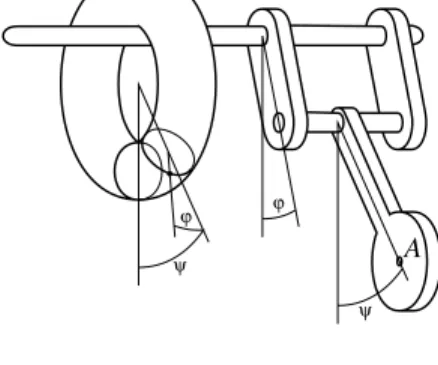
andAis defined if we knowϕand are given the eigenvector corresponding to the eigenvalue λ = 1 (two real coordinates a, b are needed for that, since eigenvectors are defined up to a scalar multiplier). Thus again three coordinates (ϕ,a,b) determine elements of SO(3), and they are Euclidean coordinates only locally.
ϕ
ϕ 1
2
Figure 1.2.
1.5. The phase space of billiards on a disk B(D2). A tiny billiard ballP moves with unit velocity in a closed diskD2, bouncing off its circular boundaryC in the natural way (angle of incidence = angle of reflection).
We want to describe the phase space B(D2) of this mechanical system, whose “points” are all the possiblestates of the system (each state being defined by the position ofP and the direction of its velocity vector). Since each state is determined by three coordinates (x, y;ϕ) (Figure 1.2), it would seem that as a set,B(D2) isD2×S1, whereS1 is the unit circle (S1 =R mod 2π). But this is not the case, because at the moment of collision with the boundary, say at (x0, y0), the direction of the velocity vector jumps fromϕ1 toϕ2 (see Figure 1.2), so that we must identify the states
(x0, y0, ϕ1)≡(x0, y0, ϕ2). (1.1)
ThusB(D2) = (D2×S1)/∼, where/∼denotes the factorization defined by the equivalence relation of all the identifications (1.1) due to all possible collisions with the boundaryC.
Since the identifications take place only on C, all the points of B0(D2) = IntD2×S1= (IntD2×S1)/∼,
where IntD2 =D2C is the interior ofD2, have neighborhoods with a structure like that of open sets in R3 (with coordinates (x, y;ϕ)). It is a rather nice fact (not obvious to the beginner) that after identifications the
“boundary states” (x, y;ϕ), (x, y) ∈C, also have such neighborhoods, so that again B(D2) is locally likeR3, but not likeR3 globally (as we shall later show).
As a more sophisticated example, the advanced reader might try to de- scribe the phase space of billiards in a right triangle with an acute angle of (a)π/6; (b) √
2π/4.
1.6. The five examples of three-dimensional manifolds described above all come from different sources: classical mechanics 1.1, algebraic geometry 1.2, classical geometry 1.3, linear algebra 1.4, and mechanics 1.5. The advanced reader has not failed to notice that 1.1–1.4 are actually examples of one and the same manifold (appearing in different garb):
Rot(3) =V =RP3= SO(3).
To be more precise, the first four manifolds are all “diffeomorphic,” i.e., equivalent as smooth manifolds (the definition is given in Section 6.7). As for Example 1.5,B(D2) differs from (i.e., is not diffeomorphic to) the other manifolds, because it happens to be diffeomorphic to the three-dimensional sphereS3(the beginner should not be discouraged if he fails to see this; it is not obvious).
What is the moral of the story? The history of mathematics teaches us that if the same object appears in different guises in various branches of mathematics and its applications, and plays an important role there, then it should be studied intrinsically, as a separate concept. That was what happened to such fundamental concepts asgroup andlinear space,and is true of the no less important concept ofsmooth manifold.
1.7. The examples show us that a manifoldM is a point set locally like Euclidean spaceRn with global structure not necessarily that ofRn. How does one go about studying such an object? Since there are Euclidean coordinates near each point, we can try to coverM withcoordinate neigh- borhoods (or charts, or local coordinate systems, as they are also called).
A family of charts covering M is called an atlas. The term is evocative;
indeed, a geographical atlas is a set of charts or maps of the manifoldS2 (the Earth’s surface) in that sense.
In order to use the separate charts to study the overall structure ofM, we must know how to move from one chart to the next, thus “gluing together”
Figure 1.3.
the charts along their common parts, so as to recoverM(see Figure 1.3). In less intuitive language, we must be in possession ofcoordinate transforma- tions, expressing the coordinates of points of any chart in terms of those of a neighboring chart. (The industrious reader might profit by actually writing out these transformations for the case of the four-charts atlas of RP3 described in 1.3.)
If we wish to obtain asmoothmanifold in this way, we must require that the coordinate transformations be “nice” functions (in a certain sense). We then arrive at thecoordinate orclassical approach to smooth manifolds. It is developed in detail in Chapter 5.
1.8. Perhaps more important is the algebraic approach to the study of manifolds. In it we forget about charts and coordinate transformations and work only with the R-algebra FM of smooth functions f: M → R on the manifold M. It turns out that FM entirely determines M and is a convenient object to work with.
An attempt to give the reader an intuitive understanding of the natural philosophy underlying the algebraic approach is undertaken in the next sections.
1.9. In the description of a classical physical system or process, the key notion is thestateof the system. Thus, in classical mechanics, the state of a moving point is described by its position and velocity at the given moment of time. The state of a given gas from the point of view of thermodynamics is described by its temperature, volume, and pressure, etc. In order to actually assess the state of a given system, the experimentalist must use variousmeasuring devices whosereadings describe the state.
Suppose M is the set of all states of the classical physical system S.
Then to each measuring deviceD there corresponds a function fD on the
set M, assigning to each state s ∈M the reading fD(s) (a real number) that the device D yields in that state. From the physical point of view, we are interested only in those characteristics of each state that can be measured in principle, so that the set M of all states is described by the collection ΦS of all functions fD, where the D’s are measuring devices (possibly imaginary ones, since it is not necessary — nor indeed practically possible — to construct all possible measuring devices). Thus, theoretically, a physical systemS is nothing more that the collection ΦS of all functions determined by adequate measuring devices (real or imagined) onS.
1.10. Now, if the functions f1, . . . , fk correspond to the measuring de- vicesD1, . . . , Dk of the physical system S, andϕ(x1, . . . , xk) is any “nice”
real-valued function ink real variables, then in principle it is possible to construct a deviceD such that the corresponding functionfD is the com- posite function ϕ(f1, . . . , fk). Indeed, such a device may be obtained by constructing an auxiliary device, synthesizing the valueϕ(x1, . . . , xk) from input entriesx1, . . . , xk (this can always be done ifϕis nice enough), and then “plugging in” the outputs (f1, . . . , fk) of the devicesD1, . . . , Dk into the inputs (x1, . . . , xk) of the auxiliary device. Let us denote this deviceD byϕ(D1, . . . , Dk).
In particular, if we take ϕ(x1, x2) = x1+x2 (or ϕ(x) = λx, λ∈ R, or ϕ(x1, x2) =x1x2), we can construct the devicesD1+D2(orλDi, orD1D2) from any given devicesD1,D2. In other words, iffi=fDi∈ΦS, then the functionsf1+f2, λfi, f1f2 also belong to ΦS.
Thus the set ΦS of all functionsf =fDdescribing the systemS has the structure of analgebra over R(orR-algebra).
1.11. Actually, the set ΦS of all functions fD : MS → R is much too large and cumbersome for most classical problems. Systems (and processes) described in classical physics are usually continuous or smooth in some sense. Discontinuous functionsfD are irrelevant to their description; only
“smoothly working” measuring devicesDare needed. Moreover, the prob- lems of classical physics are usually set in terms of differential equations, so that we must be able to take derivatives of the relevant functions from ΦS as many times as we wish. Thus we are led to consider, rather than ΦS, the smaller setFS ofsmooth functions fD:MS →R.
The setFS inherits anR-algebra structure from the inclusionFS⊂ΦS, but from now on we shall forget about Φ, since thesmooth R-algebraFS
will be our main object of study.
1.12. Let us describe in more detail what the algebra FS might be like in classical situations. For example, from the point of view of classical mechanics, a system S of N points in space is adequately described by the positions and velocities of the points, so that we need 6N measuring devicesDi to record them. Then the algebraFS consists of all elements of the formϕ(f1, . . . , f6N), where thefi are the “basic functions” determined by the devicesDi, whileϕ:R6N →Ris any nice (smooth) function.
In more complicated situations, certain relationsamong the basis func- tionsfi may arise. For example, if we are studying a system of two mass points joined by a rigid rod of negligible mass, we have the relation
3 i=1
(fi−fi+3)2=r2,
where r is the length of the rod and the functions fi (respectively fi+3) measure the ith coordinate of the first (respectively second) mass point.
(There is another relation for the velocity components, which the reader might want to write out explicitly.)
Generalizing, we can say that there usually exists a basis system of devices D1, . . . , Dk adequately describing the system S (from the chosen point of view). Then theR-algebraFS consists of all elements of the form ϕ(f1, . . . , fk), whereϕ:Rk→Ris a nice function and thefi=fDi are the relevant measurements (given by the devices Di) that may be involved in relations of the formF(f1, . . . , fk)≡0.
ThenFSmay be described as follows. LetRkbe Euclidean space with co- ordinatesf1, . . . , fk andU ={(f1, . . . , fk)|ai < fi < bi}, where the open intervals ]ai, bi[ contain all the possible readings given by the devices Di. The relationsFj(f1, . . . , fk) = 0 between the basis variablesf1, . . . , fk de- termine a surfaceMinU. ThenFSis theR-algebra of all smooth functions on the surfaceM.
1.13. Example (thermodynamics of an ideal gas). Consider a certain volume of ideal gas. From the point of view of thermodynamics, we are interested in the following measurements: the volume V, the pressure p, and the absolute temperature T of the gas. These parameters, as is well known, satisfy the relationpV =cT, wherec is a certain constant. Since 0< p <∞, 0< V <∞, and 0< T <∞, the domainU is the first octant in the spaceR3(V, p, T), and the hypersurface Min this domain is given by the equationpV =cT. The relevantR-algebraF consists of all smooth functions onM.
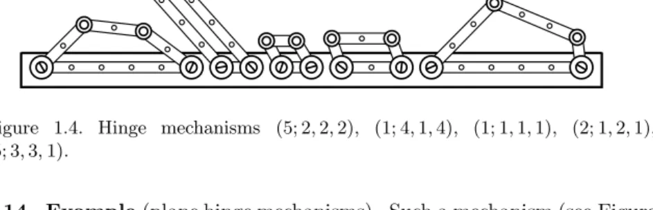
Figure 1.4. Hinge mechanisms (5; 2,2,2), (1; 4,1,4), (1; 1,1,1), (2; 1,2,1), (5; 3,3,1).
1.14. Example(plane hinge mechanisms). Such a mechanism (see Figure 1.4) consists ofn >3 ideal rods in the plane of lengths, say, (l1;l2, . . . , ln);
the rods are joined in cyclic order to each other by ideal hinges at their
endpoints; the hinges of the first rod (and hence the rod itself) are fixed to the plane; the other hinges and rods move freely (insofar as the config- uration allows them to); the rods can sweep freely over (“through”) each other. Obviously, the configuration space of a hinge mechanism is deter- mined completely by the sequence of lengths of its rods. So, one can refer to a concrete mechanism just by indicating the corresponding sequence, for instance, (5; 2,3,2). The reader is invited to solve the following problems in the process of reading the book. The first of them she/he can attack even now.
Exercise. Describe the configuration spaces of the following hinge mechanisms:
1. Quadrilaterals: (5; 2,2,2); (1; 4,1,4); (1; 1,1,1); (2; 1,2,1); (5; 3,3,1).
2. Pentagons: (3.9; 1,1,1,1); (1; 4,1,1,4); (6; 6,2,2,6); (1; 1,1,1,1).
The reader will enjoy discovering that the configuration space of (1; 1,1,1,1) is the sphere with four handles.
Exercise. Show that the configuration space of a pentagon depends only on the set of lengths of the rods and not on the order in which the rods are joined to each other.
Exercise. Show that the configuration space of the hinge mechanism (n−α; 1, . . .,1) consisting ofn+ 1 rods is:
1. The sphereSn−2 ifα= 12.
2. The (n−2)-dimensional torusTn−2=S1× · · · ×S1 ifα=32. 1.15. So far we have not said anything to explain what a states∈MS of our physical system S really is, relying on the reader’s physical intuition.
But once the set of relevant functionsFS has been specified, this can easily be done in a mathematically rigorous and physically meaningful way.
The methodological basis of physical considerations is measurement.
Therefore, two states of our system must be considered identical if and only if all the relevant measuring devices yield the same readings. Hence each states∈MS is entirely determined by the readings in this state on all the relevant measuring devices, i.e., by the correspondence FS → R assigning to each fD ∈ FS its reading (in the state s) fD(s) ∈ R. This assignment will clearly be anR-algebra homomorphism. Thus we can say, by definition, thatany statesof our system is simply an R-algebra homo- morphism s: FS →R.The set of all R-algebra homomorphismsFS →R will be denoted by|FS|; it should coincide with the setMS of all states of the system.
1.16. Summarizing Sections 1.9–1.15, we can say thatany classical phys- ical system is described by an appropriate collection of measuring devices,
each state of the system being the collection of readings that this state determines on the measuring devices.
The sentence in italics may be translated into mathematical language by means of the following dictionary:
• physical system = manifold,M;
• state of the system = point of the manifold,x∈M;
• measuring device = function onM,f ∈ F;
• adequate collection of measuring devices = smoothR-algebra,F;
• reading on a device = value of the function,f(x);
• collection of readings in the given state =R-algebra homomorphism x:F →R, f →f(x).
The resulting translation reads: Any manifold M is determined by the smooth R-algebra F of functions on it, each point x on M being the R- algebra homomorphism F → R that assigns to every function f ∈ F its valuef(x) at the pointx.
1.17. Mathematically, the crucial idea in the previous sentence is the identification of pointsx∈Mof a manifold andR-algebra homomorphisms x:F →Rof itsR-algebra of functionsF, governed by the formula
x(f) =f(x). (1.2)
This formula, read from left to right, defines the homomorphismx:F →R when the functionsf ∈ F are given. Read from right to left, it defines the functionsf:M→R, when the homomorphismsx∈M are known.
Thus formula (1.2) is right in the middle of the important duality re- lationship existing between points of a manifold and functions on it, a duality similar to, but much more delicate than, the one between vectors and covectors in linear algebra.
1.18. In the general mathematical situation, the identificationM↔ |F|
between the setMon which the functionsf ∈ Fare defined and the family of allR-algebra homomorphismsF →Rcannot be correctly carried out.
This is because, first of all,|F| may turn out to be “much smaller” than M (an example is given in Section 3.6) or “bigger” thanM, as we can see from the following example:
Example. SupposeM is the setNof natural numbers andF is the set of all functions onN(i.e., sequences {a(k)}) such that the limit limk→∞a(k) exists and is finite. Then the homomorphism
α:F →R, {a(k)} → lim
k→∞a(k), does not correspond to any point ofM=N.
Indeed, ifαdid correspond to some pointn∈N, we would have by (1.2) n(a(·)) =a(n),
so that
klim→∞a(k) =α(a(·)) =n(a(·)) =a(n)
for any sequence {a(k)}. But this is not the case, say, for the sequence ai = 0, in, ai = 1, i > n. Thus|F| is bigger thanM, at least by the homomorphismα.
However, we can always add to N the “point at infinity” ∞ and ex- tend the sequences (elements ofF) by puttinga(∞) = limk→∞a(k), thus viewing the sequences inF as functions onN∪ {∞}. Then obviously the homomorphism above corresponds to the “point”∞.
This trick of adding points at infinity (or imaginary points, improper points, points of the absolute, etc.) is extremely useful and will be exploited to great advantage in Chapter 8.
1.19. In our mathematical development of the algebraic approach (Chap- ter 3) we shall start from an R-algebra F of abstract elements called
“functions.” Of course, F will not be just any algebra; it must meet cer- tain “smoothness” requirements. Roughly speaking, the algebraFmust be smooth in the sense that locally (the meaning of that word must be defined in abstract algebraic terms!) it is like theR-algebraC∞(Rn) of infinitely differentiable functions inRn. This will be the algebraic way of saying that the manifoldM is locally like Rn; it will be explained rigorously and in detail in Chapter 3. When the smoothness requirements are met, it will turn out thatF entirely determines the manifoldM as the set |F|of all R-algebra homomorphisms of F intoR, andF can be identified with the R-algebra of smooth functions on M. The algebraic definition of smooth manifold appears in the first section of Chapter 4.
1.20. Smoothness requirements are also needed in the classical coordi- nate approach, developed in detail below (see Chapter 5). In particular, coordinate transformations must be infinitely differentiable. The rigorous coordinate definition of a smooth manifold appears in Section 5.8.
1.21. The two definitions of smooth manifold (in which the algebraic ap- proach and the coordinate approach result) are of course equivalent. This is proved in Chapter 7 below. Essentially, this book is a detailed exposition of these two approaches to the notion of smooth manifold and their equiv- alence, involving many examples, including a more rigorous treatment of the examples given in Sections 1.1–1.5 above.
2
Cutoff and Other Special Smooth Functions on R n
2.1. This chapter is an auxiliary one and can be omitted on first reading.
In it we show how to construct certain specific infinitely differentiable func- tions on Rn (the R-algebra of all such functions is denoted byC∞(Rn)) that vanish (or do not vanish) on subsets ofRnof special form. These func- tions will be useful further on in the proof of many statements, especially in the very important Chapter 3.
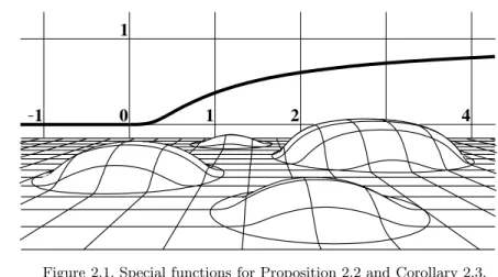
2.2 Proposition. There exists a functionf ∈C∞(R)that vanishes for all negative values of the variable and is strictly positive for its positive values.
We claim that such is the function f(x) =
0 forx0,
e−1/x forx >0 (2.1) (see Figure 2.1 in the background). The only thing that must be checked is thatf is smooth, i.e.,f ∈C∞(R).
By induction overn, we shall show that thenth derivative off is of the form
f(n)(x) =
0 forx0,
e−1/xPn(x)x−2n forx >0, (2.2) wherePn(x) is a polynomial, and thatf(n)is continuous.
Forn= 0 this is obvious, since limx→+0e−1/x= 0.
1
1
0 1 2 4
Figure 2.1. Special functions for Proposition 2.2 and Corollary 2.3.
If (2.2) is established for somen0, then obviouslyf(n+1)(x) = 0 when x <0, while if x >0, we have
f(n+1)(x) =e−1/x
Pn(x) +x2Pn(x)−2nxPn(x)
x−2n−2, which shows thatf(n+1)is of the form (2.2).
To show that it is continuous, note that limx→+0e−1/xxα = 0 by L’Hospital’s rule for any realα. Hence limx→+0f(n+1)(x) = 0 and (again by L’Hospital’s rule)
f(n+1)(0) = lim
x→0
f(n)(x)−f(n)(0)
x = lim
x→0
f(n+1)(x)−0
1 ,
so thatf(n+1) equals 0 forx0 and is continuous for allx.
Exercise. Letf be the function defined in (2.1) and letck = maxf(k). 1. Prove thatck <∞for allk.
2. Investigate the behavior of the sequence{ck}whenk→ ∞.
2.3 Corollary. For any r > 0 and a ∈ Rn there exists a function g ∈ C∞(Rn)that vanishes for allx∈Rn satisfyingx−arand is positive for all otherx∈Rn.
Such is, for example, the function g(x) =f
r2− x−a2 ,
wheref is the function (2.1) from Section 2.2 (see Figure 2.1).
2.4 Proposition. For any open set U ⊂Rn there exists a function f ∈ C∞(Rn)such that
f(x) = 0, ifx /∈U, f(x)>0, ifx∈U.
Special Smooth Functions onR 15 If U =Rn, take f ≡1; ifU = ∅, take f ≡ 0. Now suppose U = Rn, U =∅, and let{Uk}be a covering of U by a countable collection of open balls (e.g., all the balls of rational radius centered at the points with rational coordinates and contained in U). By Corollary 2.3, there exist smooth functionsfk ∈ C∞(Rn) such that fk(x) >0 if x ∈ Uk and fk(x) = 0 if x /∈Uk. Put
Mk = sup
p1+···+p0pkn=p x∈Rn
∂pfk
∂p1x1· · ·∂pnxn(x) .
Note that Mk < ∞, since outside the compact set Uk (the bar denotes closure) the functionfk and all its derivatives vanish.
Further, the series
∞ k=1
fk 2kMk
converges to a smooth functionf, since for allp1, . . . , pn the series ∞
k=1
fk
2kMk
∂p1+···+pnfk
∂xp11· · ·∂xpnn
converges uniformly (because wheneverkp1+· · ·+pn, the absolute value of thekth term is no greater than 2−k).
Clearly, the function f possesses the required properties.
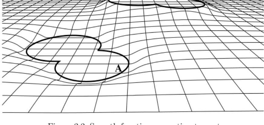
2.5 Corollary. For any two nonintersecting closed sets A, B⊂Rn there exists a functionf ∈C∞(Rn)such that
f(x) = 0, whenx∈A;
f(x) = 1, whenx∈B;
0< f(x)<1, for all otherx∈Rn.
Using Proposition 2.4, choose a function fA that vanishes on A and is positive outsideAand a similar functionfB forB. Then forf we can take the function
f = fA
fA+fB
(see Figure 2.2).
2.6 Corollary. Suppose U ⊂Rn is an open set and f ∈ C∞(U). Then for any point x ∈ U there exists a neighborhood V ⊂ U and a function g∈C∞(Rn)such that f
V ≡g
V.
SupposeW is an open ball centered atxwhose closure is contained inU. LetV be a smaller concentric ball. The required functiongcan be defined
A B
Figure 2.2. Smooth function separating two sets.
as
g(y) =
h(y)·f(y), wheny∈U, 0, wheny∈Rn\U,
where the functionh∈C∞(Rn) is obtained from Corollary 2.3 and satisfies h
V ≡1, h
Rn\W ≡0.
2.7 Proposition.On any nonempty open setU ⊂Rn there exists a smooth function with compact level surfaces,i.e.,a function f∈C∞(U)such that for anyλ∈Rthe set f−1(λ)is compact.
Denote by Ak the set of points x∈ U satisfying both of the following conditions:
(i) xk,
(ii) the distance from x to the boundary of U is not less than 1/k (if U =Rn, then condition (ii) can be omitted).
Obviously, all points ofAk are interior points ofAk+1. Hence Ak and the complement inRn to the interior of the setAk+1 are two closed noninter- secting sets. By Corollary 2.5 there exists a function fk ∈ C∞(Rn) such
that
fk(x) = 0 ifx∈Ak, fk(x) = 1 ifx /∈Ak+1, 0< fk(x)<1 otherwise.
Since any point x ∈ U belongs to the interior of the set Ak for all sufficiently largek, the sum
f = ∞ k=1
fk
Special Smooth Functions onR 17 is well defined, andf is smooth onU (locally it is a finite sum of smooth functions).
Consider a pointx∈U\Ak. Since all the functionsfi are nonnegative, and fori < k we havefi(x) = 1, it follows that f(x)k−1. Hence, for anyλ∈Rthe set f−1(λ) is a closed subset of the compact set Ak, where k is an integer such thatλ < k−1. A closed subset of a compact set is always compact, so thatf is the required function.
Let us fix a coordinate systemx1, . . . , xnin a neighborhoodU of a point z. Recall that a domainU is called starlike with respect to z if together with any pointy∈U it contains the whole interval (z, y).
2.8 Hadamard’s lemma. Any smooth functionf in a starlike neighbor- hood of a pointz is representable in the form
f(x) =f(z) + n i=1
(xi−zi)gi(x), (2.3) wheregi are smooth functions.
In fact, consider the function
ϕ(t) =f(z+ (x−z)t).
Thenϕ(0) =f(z) and ϕ(1) =f(x), and by Newton–Leibniz formula, ϕ(1)−ϕ(0) =
1 0
dϕ dtdt=
1 0
n i=1
∂f
∂xi
(z+ (xi−zi)t)(xi−zi)dt
= n i=1
(xi−zi) 1
0
∂f
∂xi
(z+ (xi−zi)t)dt.
Since the functions
gi(x) = 1
0
∂f
∂xi
(z+ (xi−zi)t)dt
are smooth, this concludes the proof of Hadamard’s lemma.
Let, as before, x1, . . . , xn be a fixed coordinate system of a pointz in a neighborhoodU and letτ= (i1, . . . , in) be a multi-index. Set
|τ|=i1+· · ·+in, ∂|τ|
∂xτ = ∂|τ|
∂xi11· · ·∂xinn
, (x−z)τ= (x1−z1)i1· · ·(xn−zn)in, τ! =i1!· · ·in!.
2.9 Corollary. (Taylor expansion in Hadamard’s form.)Any smooth func- tion f in a starlike neighborhood U of a point z is representable in the form
f(x) = n
|τ|=0
1
τ!(x−z)τ∂|τ|f
∂xτ (z) +
|σ|=n+1
(x−z)σgσ(x), (2.4)