ISSN: 1693-6930
accredited by DGHE (DIKTI), Decree No: 51/Dikti/Kep/2010 191
Efficient Motion Field Interpolation Method for
Wyner-Ziv Video Coding
I Made Oka Widyantara*1, Wirawan2, Gamantyo Hendrantoro3 1
Department of Electrical Engineering, Universitas Udayana, Denpasar Bali, Indonesia
2,3Department of Electrical Engineering, Institut Teknologi Sepuluh Nopember (ITS), Surabaya, Indonesia
e-mail: [email protected]*1, [email protected], [email protected]
Abstrak
Sandi video Wyner-Ziv mampu menurunkan kompleksitas penyandian video dengan memindahkan prosedur estimasi gerak dari penyandi ke pengawasandi. Di antara beberapa metode motion estimation yang telah diterapkan, algoritma expectation maximization adalah yang paling efektif. Sayangnya, penerapan estimasi gerak berbasis blok pada algoritma ini menyebabkan profil bidang gerak dibatasi oleh granularitas ukuran blok. Kasus serupa dalam pengkodean multiview, diselesaikan menggunakan interpolasi tetangga-terdekat dan bilinear. Paper ini bermaksud mengevaluasi penerapan metode interpolasi tersebut pada codec video Wyner-ziv kawasan transformasi dengan melihat kinerja pada penghematan laju bit, laju-distorsi dan kompleksitas pengawasandian. Hasil riset menunjukan interpolasi bilinear hanya efektif diterapkan untuk pemrosesan sekuen video pergerakan tinggi. Pada video pergerakan tinggi, penghematan laju bit mencapai 3.29%, PSNR lebih tinggi 0,2 dB, dan kompleksitas pengawasandian yang ditimbulkan lebih tinggi sebesar 12,30% dibandingkan dengan interpolasi tetangga-terdekat. Pada video pergerakan lambat, penghematan laju bit hanya mencapai 0,82 %, dengan hampir tanpa perubahan PSNR, sedangkan kompleksitas pengawasandian meningkat sampai 10,32%.
Kata kunci: bilinear, interpolasi bidang gerak, tetangga-terdekat, Wyner-Ziv video coding
Abstract
Wyner-Ziv video coding has the capability to reduce video encoding complexity by shifting motion estimation procedure from encoder to decoder. Amongst many motion estimation methods, expectation maximization algorithm is the most effective one. Unfortunately, the implementation of block-based motion estimation in this algorithm causes motion field profile bounded by granularity of block size. Nearest-neighbor and bilinear interpolation methods have already applied in multiview image coding to handle similar problem. This paper aims to evaluate performance of both interpolation methods in transform-domain Wyner-Ziv video codec. Results showed that bilinear interpolation effective only for high motion video sequences. In this scenario, it hasbitrate saving up to 3.29 %, 0.2 dB higher PSNR, and 12.30 % higher decoding complexity compared to nearest-neighbor. In low motion video content, bitrate saving only gained up to 0.82%, with almost the same PSNR, while decoding complexity increase up to 10.32%.
Keywords: bilinear, motion field interpolation, nearest-neighbor, Wyner-Ziv video coding
1. Introduction
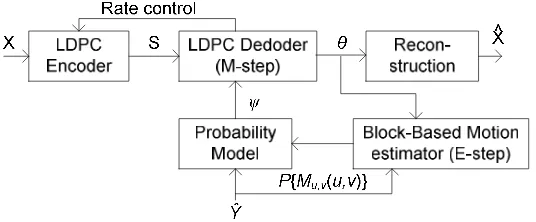
Wyner-Ziv video coding (WZVC) is a new paradigm in video coding [1], based on Slepian-Wolf [2] and Wyner-Ziv [3] information theories in 1970s. Those theories proved that separate encoding and joint decoding (distributed compression) can achieve similar performances to joint encoding and joint decoding as long as correlated side information (SI) is used in decoder side. Model of this approach is shown in Figure 1, where SI is received by exploit correlation between frames that already been decoded.
SI quality strongly influences the compression efficiency in WZVC system. In general, better SI will lead to better rate-distortion (RD) performance. But, as long as SI is generated in decoder with minimum information about source, accurate SI estimation becomes a difficult task. So, to enhance WZVC performance, the principal investigators of the DISCOVER project identify “ finding the best SI at the decoder” as a key task [4].
current frame by motion estimation that uses decoded frame. However, decoded frame carries only limited information. Moreover, since blind motion estimation does not use any information of current frame to be encoded, the SI is generally not accurate. Discover codec follows this WZVC architecture and improves SI generation to increase system performance [5]-[7]. In this codec, estimate of motion field within MCI is done bidirectionally (backward and forward motion estimation) followed by spatial motion smoothing technique to smoothen blocking effect.
More recently, SI generation method by motion vector learning along decoding process using expectation maximization (EM) algorithm for WZVC system has been proposed by [8]. The same method had been applied for learning disparity information in distributed coding of random dot stereograms [9] and distributed grayscale stereo image coding [10], [11]. Learning based method using EM algorithm does disparity compensation and motion field compensation based on block, where disparity and motion field profile bounded by granularity of k-by-k blocks. To improve disparity estimate, a disparity block-to-pixel Interpolation method using bilinear interpolation had been proposed by [12]. This approach gains significant bit saving compared to nearest-neighbor (NN) interpolation previously applied. However, bilinear interpolation increases decoding complexity, since it uses more spatial blocks for weighting factors.
This paper aims to evaluate implementation of disparity probability interpolation [12] in WZVC codec [8] by interpolate motion field distribution from block to pixel. The differences of motion field characteristic between sequence of video frames allow design of WZVC codec to implement different interpolation methods. The main contribution of this paper is to find efficient motion field distribution interpolation method from block to pixel in WZVC codec [8], for video sequences of different motion characteristics, in the sense of saving bitrate, RD performance, and decoding complexity.
This paper is organized as follows. In section 2, unsupervised forward motion vector learning based on EM algorithm [8] for WZVC codec is reviewed. Next on section 3, EM algorithm for unsupervised forward motion vector learning with motion field distribution interpolation method from block to pixel is extended. Evaluation of this implementation method in transform-domain WZVC [8] will be explained in section 4, and finally conclusions are presented in section 5.
Slepian-Wolf Encoder
Conventional Encoder Separate
encoding
Conventional Decoder Slepian-Wolf
Decoder
Side Information
Joint decoding Rate
R > H(X|Y) X
Y
X^
Y
Figure 1. Distributed compression : separate encoding and joint decoding
2. EM-Based Unsupervised Forward Motion Vector Learning for WZVC
The main objective of EM algorithm is to estimate parameter without any prior information or complete observation data. EM algorithm ensures that estimate coefficient converges to local optimized value using maximum likelihood function. EM algorithm frame work to find forward motion vector in WZVC codec is shown in Figure 2. Below are details of EM algorithm that used in [8].
2.1. Model
In Figure 2, X is current Wyner-Ziv luminance frame and Ŷ is previously decoded
luminance frame, where X is related to Ŷthrough a forward motion field M. The residual of X with respect to motion-compensated Ŷ is treated as independent Laplacian noise Z. So, the decoder’s a posteriori probabilty distribution of source X based on parameter θ, can be modeled
as below:
{ } { }
= =∏
(
( )
)
j i
app X P X i j X i j
P
,
, , ,
;
θ
θ
(1)where θ(i,j,ω) = Papp{X(i,j) = ω} is “soft estimate” of X(i,j) in luminance values ω∈{ 0,..., 2 d
-1} and d is bit depth.
2.2. Problem
The decoder aims to calculate the a posteriori probability distribution of motion,
{ }
M
P
{
M
|
Y
ˆ
,
S
;
θ
}
P
{ }
M
P
{
Y
ˆ
,
S
|
M
;
θ
}
P
app≡
∝
(2)with the second step by Bayes’ Law. The form of this expression suggests an iterative EM solution. The E-step updates the motion field distribution with reference to the source model parameters, while the M-step updates the source model parameters with reference to the motion field distribution. Note that P{M|Y,S;θ} is the probability of observing motion M given that
it relates X (as parameterized byθ) to Ŷ, and also given syndrome S.
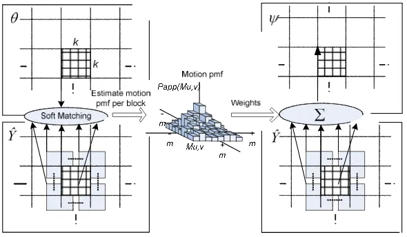
2.3. E-step Algorithm
The E-step updates the estimated distribution on M and before renormalization is written as
{ }
( 1){ }
{
( 1)}
) (
;
|
,
ˆ
−−
=
t tapp t
app
M
P
M
P
Y
S
M
P
θ
(3)To reduce operational cost from possibly high value of M, motion field estimation of M is conducted by block-by-block motion vectors Mu,v.For a specified blocksize k, every k-by-k block
of θ(t−1)
is compared to the colocated block of Ŷ as well as all those in a fixed motion search
range around it (± m pixels horizontally and vertically, respectively). For a block θu,v (t-1)
with top left pixel located at (u,v), the distribution on the shift Mu,vis updated as below and normalized:
{ }
{ }
{
( 1)}
, , )
, ( , ) 1 ( ,
) (
;
|
ˆ
:
,
− +
−
=
tv u v u M v u v u t app v
u t
app
M
P
M
P
Y
M
P
v
u
θ
(4)where Ŷ(u,v)+Mu,v is the k-by-k block of Ŷ with top left pixel at ((u,v)+Mu,v). Note that
P{Ŷ(u,v)+Mu,v|Mu,v;θu,v(t-1)
} is the probability of observing Ŷ(u,v)+Mu,v given that it was generated
through vector Mu,vfrom Xu,v as parameterized by θu,v
(t-1)
. This procedure, shown in the left of Figure 3, occurs in the block-based motion estimator.
2.4. M-step
The M-step updates the soft estimate θ by maximizing the likelihood of Ŷ and
( ) =
{
Θ}
=∑
{
=}
{
= Θ}
ΘΘ m
t app t
m M S Y P m M P S
Y
P ˆ, ; argmax ˆ, | ;
max arg
: ()
θ
(5)where, the summation is over all configurations m of the motion field. Since true maximization is intractable, an approach is conducted by generating soft SI ψ(t), followed by an iteration of joint bitplane low-density parity-check (LDPC) decoding to yield θ(t)
. The process can be distinguished as follows:
Generating Soft SI (ψψψψ(t)).In this step, soft SI ψ(t)u,v is created by blending estimates from each
the blocks Ŷ(u,v)+Mu,v according to Papp(t)
{Mu,v} as shown in the probability model in the right hand
side of Figure 3. More generally, the probability that the blended SI has value ! at pixel (i, j) is
(
)
=∑
{
=}
{
= =}
m t app t
Y m M j
i X P m M P j
i, , () (, ) | ,ˆ
)
(
ω
ω
ψ
{
}
(
ˆ (, ))
) (
j i Y p m M
P Z m
m t
app = −
=
∑
ω
(6)where pZ(z) is the probability mass function of the independent additive noise Z, and Ŷm is the
previous reconstructed frame compensated through motion configuration m.
Figure 3. E-step block-based motion estimator (left) and probability model (right)
Generating soft estimate (θ(t)). Soft SI (ψ(t)). generated by model probability then used by
LDPC decoder to generate soft estimate (θ(t)
). To this process, LDPC decoder implement joint bit plane LDPC decoding method to maximize soft SI ψ(t)(i,j,!) and syndrome (S). For procedure in detail of joint bitplane algorithm decoding, please refere to [8].
2.5. Termination
Iterating between the E-step and the M-step in this way learns the forward motion vectors at the granularity of k-by-k blocks. The decoding algorithm terminates successfully when the hard estimates
X
ˆ
(
i
,
j
)
=
arg
max
ωθ
(
i
,
j
,
ω
)
yield a syndrome equal to S3. Research Method
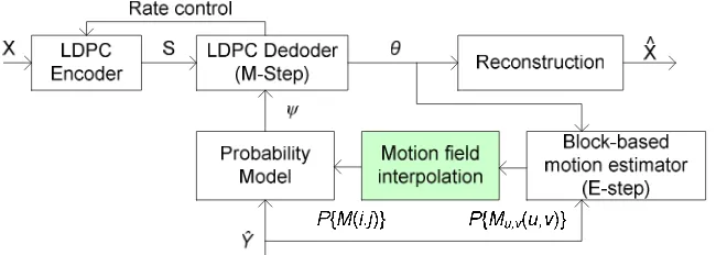
To increase soft SI ψ(t), we have to improve motion field profile (M) in order to minimize effect of unnatural step–like transitions in block boundaries. This improvement carried out by computing motion field distribution in pixel based Papp{M(i,j)} to estimate motion field (M)
boundaries. This approach is equivalent with interpolate motion field distribution from block to pixel.
As described in Equation (6) of section 2, pixel-based motion field distribution Papp{M(i,j)} then used as weighting factor for probability mass function of independent additive
noise pZ(z) in soft SI ψ
(t)
generation process. This soft SI ψ(t) accuracy is mainly depend on distribution Papp{M(i,j)}. Improvement process will be done in the every EM iteration. For this
aproach, a motion field interpolation process is added after block-based motion estimator in WZVC. Framework of EM algorithm with motion field interpolation in WZVC is shown in Figure 4.
In paper [12] on Wyner-Ziv coding of stereo image with unsupervised learning of disparity, disparity improvement is carried out by applying bilinear interpolation and the results are compared to NN interpolation applied in [9,10,11]. This approach gave significant bit saving, however there was no explanation about decoding complexity as the consequences of that approach.
In distributed video coding application, different characteristic of motion field (M) between sequence of video frames allow WZVC codec to implement different interpolation methods. This paper adopts NN and bilinear interpolation [12] to improve motion field (M) estimation and to compare their performances in WZVC codec [8] for different video sequence input. More details of implementation of interpolation method in [12] are discussed in sections below.
Figure 4. Motion field interpolation in EM-based unsupervised forward motion vector learning for WZVC
3.1. Nearest-Neighbor(NN)Interpolation
In motion field interpolation from block to pixel, NN interpolation method only computes single blockwise motion field distribution Papp{Mu,v} for every pixel within k-by-k block. So all
pixels in this block shares the same blockwise motion field distribution Papp{Mu,v}. If Mu,v(u,v) is
denotes block-by-block motion field and M(i,j) denotes pixel-by-pixel motion field, pixel-by-pixel motion field distribution motion field defines as
( )
{
}
= jk
k i M P j i M
Pt appt uv
app , , ,
) ( )
( (7)
where k is the block size.
When there is a high correlation between blocks in frame X with blocks in previously decoded frame Ŷ, motion field estimation generated by block-based motion estimation will be
more accurate. This condition allows single blockwise motion field distribution Papp{Mu,v} to be
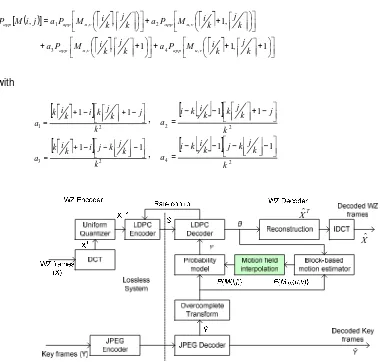
3.2. Bilinear Interpolation
In bilinear interpolation, motion field interpolation from block to pixel computes 4 (four) blockwise motion field distribution for every pixel in k-by-k block. As stated in Equation (8), each distribution has weighting factor a1to a4, where those weighting factors are chosen such as the
closest block spatially contributes more to the weighted sum. Also, a1 through a4 are properly
normalized by the area of the k-by-k block so that bilinear interpolation creates a convex combination of the disparity probabilities.
( )
[
]
+
+ + + + + + = 1 , 1 1 , , 1 , , , 4 , 3 , 2 , 1 k j k i M P a k j k i M P a k j k i M P a k j k i M P a j i M P v u app v u app v u app v u appapp (8)
with
[
]
2 1 1 1 k j k j k i k i k a + − − + = ,
[
]
2 2 1 1 k j k j k k i k i a + − − − =
[
]
2 3 1 1 k k j k j i k i k a − − − + = ,
[
]
2 4 1 1 k k j k j k i k i a − − − − = T Xˆ XˆFigure 5. Architecture of transform-domain WZVC codec
4. Results and Analysis
Procedure of motion field interpolation in EM-based unsupervised forward motion vector learning is shown in Figure 4. We implement it in transform-domain WZVC codec as in [8], with codec architecture shown in Figure 5. Codec divides video sequence into fixed size group of picture (GOP). The first frame in GOP is coded as Key frame using JPEG standard and decoded without any reference to SI. The subsequent frames of GOP (called WZ frames) are coded according to Figure 6 using previous reconstructed frame as decoder reference.
are then quantized uniformly using JPEG quantization with scale factor of 0.5, 1, 2, and 4 [15]. Quantization indices are input into LDPC encoder to reconstruct syndrome (S).
After 50 decoding iterations of EM, if the reconstructed
X
ˆ
still does not satisfy the syndrome condition, the decoder requests additional incremental transmission from the encoder via a feedback channel.(a) (b) (c) (d)
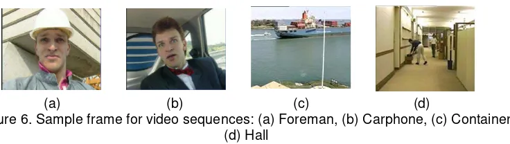
Figure 6. Sample frame for video sequences: (a) Foreman, (b) Carphone, (c) Container, (d) Hall
In DCT procedures, we use block size of 8 x 8 pixels for the block-based motion estimatior, the motion field interpolation, and the probability model. To estimate block-based motion field in motion estimator and probability model, we use motion search range ± 5 pixels horisontally and vertically. Rate control is impelemented by using rate-adaptive regular degree 3 LDPC accumulate codes of length 50688 bits as a platform for the joint bitplane systems. In these experiments, the EM algorithm at the decoder is initialized with a good value for variance of Laplacian noise Z and experimentally-chosen distributions for motion vectors Mu,v:
{ }
( )
( )
∗ ∗ = ⋅
= =
otherwise M
if
M if M
P uv
v u
v u t app
,
) 0 , ( ), , 0 (
) 0 , 0 ( ,
2 80
1
, 80
1 4 3
, 2
4 3
, )
(
(9)
4.1. Analysis of bitrate savings
Table 1 shows a comparison of average bitrate that needed to transmit WZ frame when WZVC decoder uses NN and bilinear motion field interpolations. In general, bilinear interpolation yields saving rate in all quantization factors. However, when decoding complexity is considered, only Foreman and Carphone video sequences give significant saving bitrate, i.e. up to 3.29% and 2.73% respectively, at Q0.5 quantization scaling factor. For decoding complexities, both video sequences increase up to 12.30% and 9.74%, respectively. This results show that bilinear interpolation has the capability to improve initial motion field for high motion content video sequence. Four selected weighting coefficients are able to make spatially closer blocks to source pixel contribute more to the weighted sum in smoothen motion field profile.
On the contrary, for low motion video sequence, i.e. Container and Hall, saving bitrate achieved by bilinear interpolation is not worth compared to it’s complexity. Both video sequences gain only 0.82% and 0.92%, respectively, while decoding complexities increase up to 10.32% and 15.35%, respectively at Q0.5. So, when decoding complexity becomes major concern, NN interpolation is more suitable to improve motion field estimation in WZVC codec for low motion video sequence.
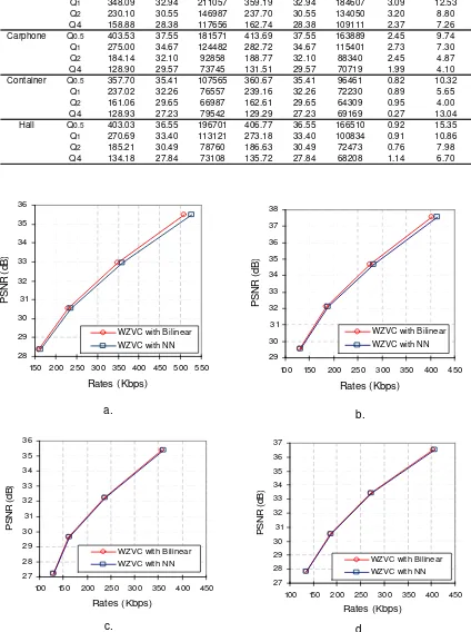
4.2. Analysis of Rate-Distortion Performance
Table 1. Comparison of transform-domain WZVC codec in different interpolation methods
Rate (kbps)
PSNR (dB)
Decoding time (s)
Rate (kbps)
PSNR (dB)
Decoding time (s)
a b c d e f (d-a)/d (c-f)/c Foreman Q0.5 509.63 35.49 289714 526.96 35.49 254077 3.29 12.30 Q1 348.09 32.94 211057 359.19 32.94 184607 3.09 12.53 Q2 230.10 30.55 146987 237.70 30.55 134050 3.20 8.80 Q4 158.88 28.38 117656 162.74 28.38 109111 2.37 7.26 Carphone Q0.5 403.53 37.55 181571 413.69 37.55 163889 2.45 9.74 Q1 275.00 34.67 124482 282.72 34.67 115401 2.73 7.30 Q2 184.14 32.10 92858 188.77 32.10 88340 2.45 4.87 Q4 128.90 29.57 73745 131.51 29.57 70719 1.99 4.10 Container Q0.5 357.70 35.41 107565 360.67 35.41 96461 0.82 10.32
Q1 237.02 32.26 76557 239.16 32.26 72230 0.89 5.65 Q2 161.06 29.65 66987 162.61 29.65 64309 0.95 4.00 Q4 128.93 27.23 79542 129.29 27.23 69169 0.27 13.04 Hall Q0.5 403.03 36.55 196701 406.77 36.55 166510 0.92 15.35 Q1 270.69 33.40 113121 273.18 33.40 100834 0.91 10.86 Q2 185.21 30.49 78760 186.63 30.49 72473 0.76 7.98 Q4 134.18 27.84 73108 135.72 27.84 68208 1.14 6.70
Saving rate (%)
Decoding complexity
(%) Video
Sequences
Scaling factor Q
WZVC with Bilinear Interpolation WZVC with NN Interpolation
a. b.
c. d.
Figure 7. RD performance comparison of transform-domain WZVC codec for NN and bilinear interpolation: a Foreman, b. Carphone, c. Container, d. Hall
29 30 31 32 33 34 35 36 37 38
100 150 200 250 300 350 400 450
Rates (Kbps)
P
S
N
R
(
d
B
)
WZVC with B ilinear WZVC with NN
27 28 29 30 31 32 33 34 35 36
100 150 200 250 300 350 400 450 Rates (Kbps)
P
S
N
R
(
d
B
)
WZVC with B ilinear WZVC with NN
27 28 29 30 31 32 33 34 35 36 37
100 150 200 250 300 350 400 450 Rates (Kbps)
P
S
N
R
(
d
B
)
WZVC with B ilinear WZVC with NN 28
29 30 31 32 33 34 35 36
150 200 250 300 350 400 450 500 550 Rates (Kbps)
P
S
N
R
(
d
B
)
4.3. Decoding complexity
To estimate decoding complexity, total decoding time for all sequences is measured in seconds. Table 1 shows total time needed to encode all 96 frames using JPEG quantization matrix at scale of Q0.5, Q1, Q2 and Q3. In general, experiment results show that implementation of bilinear interpolation makes decoding process of transform-domain WZVC codec becomes more complex. Regarding to decoding complexity, bilinear interpolation is more efficient for video sequence with high motion content, such as Foreman and Carphone. Meanwhile, for low motion content video sequence like Container and Hall, NN interpolation is more efficient to implement.
5. Conclusions
This paper has evaluated implementation of motion field interpolation method in transform-domain WZVC codec that use block-based motion field compensation method at each EM algorithm iteration. Motion field quality improvement was carried out by motion field block to pixel interpolation using NN and bilinear interpolation methods. Performances of implementation of both interpolations in transform-domain WZVC codec were analyzed based on saving bitrate, RD performance, and decoding complexity. Experiment results showed that bilinear interpolation gave more efficient saving bitrate, RD performance, and decoding complexity for video sequence with high motion content, while NN interpolation achieved almost equal saving bitrate and RD performance to bilinear interpolation for low motion content, but far lower decoding complexity.
For further work, we will implement super-sampling interpolation to increase transform-domain WZVC codec performances, mainly in processing video sequence with high motion content.
Acknowledgment
The authors would like to thank David Varodayan and David Chen of Information System Lab., Department of Electrical Engineering at Stanford University for sharing the code of WZVC codec. This work has been supported by the Directorate General of Higher Education (DGHE), Ministry of National Education Republic of Indonesia.
References
[1]. Bern G, Anne A, Shantanu R, David RM. Distributed Video Coding. Proceedings of the IEEE. 2005; 93: 71–83.
[2]. David. S, Jack KW. Noiseless Coding of Correlated Information Sources.IEEE Transaction Information Theory. 1973; 19(4): 471– 480.
[3]. Aaron DW, Jacob Z. The Rate-Distortion Function for Source Coding with Side Information at the Dekoder. IEEE Transaction. Information Theory. 1976; 22(1): 1–10.
[4]. Christine G, Fernando P, Luis T, Touradj E, Riccardo L, Jöern O. Distributed monoview and multiview video coding. IEEE Signal Processing Magazine. 2007: 24(5): 67-76.
[5]. Xavier A, Joäo A, M Dalai, S Klomp, Denis K, and Mourad O. The DISCOVER codec: Architecture, Techniques and Evaluation. Proceedings of Picture Coding Symposium. Lisbon, Portugal, 2007.
[6]. Joäo A, Catarina B, Fernando P. Improving Frame Interpolation With Spatial Motion Smoothing For Pixel Domain Distributed Video Coding. Proceedings of EURASIP Conference Speech Image Processing, Multimedia Commuication Services. Smolenice, Slovak Republic. 2005.
[7]. Joäo A, Catarina B, Fernando P. Content Adaptive Wyner-Ziv Video Coding Driven by Motion Activity. Proceedings of IEEE International Conference Image Processing. Atlanta, Georgia. 2006.
[9]. David V, Aditya M, Markus F, Bern G. Distributed Coding of Random Dot Stereograms with Unsupervised Learning of Disparity. Proceedings of IEEE International Workshop Multimedia Signal Processing. Victoria, BC, Canada. 2006.
[10]. David V, Aditya M, Markus F, Bern G. Distributed Grayscale Stereo Image Coding with Unsupervised Learning of Disparity. Proceedings of IEEE Data Compression Conference. Snowbird, UT. 2007
[11]. David V, Yao CL, Aditya M, Markus F, Bernd G.,Wyner-Ziv Coding of Stereo Image with Unsupervised Learning of Disparity. Proceedings of Picture Coding Symposium. Lisbon, Portugal. 2007
[12]. David C, David V, Markus F, Bern G. Distributed Stereo Image Coding with Improved Disparity and Noise Estimation. Proceedings of IEEE International Conference on Acoustics, Speech, and Signal Processing. Las Vegas, Nevada. 2008
[13]. Angelos L, Zixiang X, Costas G. Compression of binary sources with side information at the dekoder using LDPC codes. IEEE Commun. Letter. 2002; 6 (10):440–442.
[14]. David. C, David V, Markus F, Bern G. Wyner-Ziv coding of multiview images with unsupervised learning of disparity and Gray code. Proceedings of IEEE International Conference Image Processing. San Diego, CA, 2008.