CONCLUSION STOCK RETURN VOLATILITY AND COINTEGRATION OF U.S. AND ASIAN MARKETS IN ACCORDANCE WITH THE FINANCIAL CRISIS (1997-2014).

(1)

CHAPTER V

CONCLUSION

5.1.

Conclusion

This study objectives is to examine the stock return volatility in four asian countries from July 1997 until June 2014. By employed the GARCH models as the tool, the cyclical nature of the stock can be examined. Based on the results it can be

concluded that there‟s increases in return during good times is connected with the

decreases in volatility and the decreases in return during bad times is connected with

the increases in volatility. And also based on the analysis it shows that there‟s a

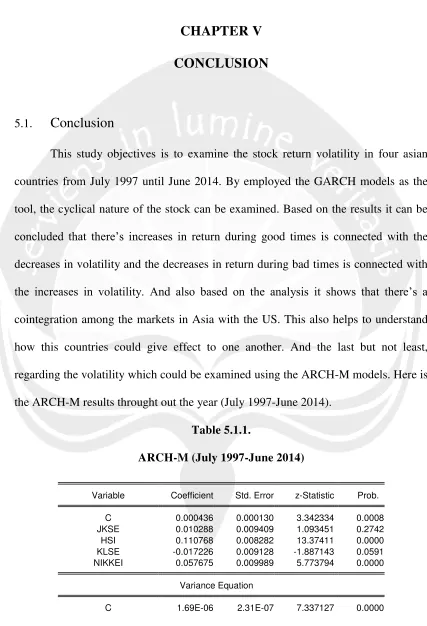
cointegration among the markets in Asia with the US. This also helps to understand how this countries could give effect to one another. And the last but not least, regarding the volatility which could be examined using the ARCH-M models. Here is the ARCH-M results throught out the year (July 1997-June 2014).

Table 5.1.1.

ARCH-M (July 1997-June 2014)

Variable Coefficient Std. Error z-Statistic Prob.

C 0.000436 0.000130 3.342334 0.0008 JKSE 0.010288 0.009409 1.093451 0.2742 HSI 0.110768 0.008282 13.37411 0.0000 KLSE -0.017226 0.009128 -1.887143 0.0591 NIKKEI 0.057675 0.009989 5.773794 0.0000

Variance Equation

(2)

RESID(-1)^2 0.094022 0.006231 15.09013 0.0000 GARCH(-1) 0.893288 0.007006 127.5067 0.0000

R-squared 0.049683 Mean dependent var 0.000182 Adjusted R-squared 0.048825 S.D. dependent var 0.012429 S.E. of regression 0.012122 Akaike info criterion -6.423924 Sum squared resid 0.650960 Schwarz criterion -6.412385 Log likelihood 14253.05 Hannan-Quinn criter. -6.419855 Durbin-Watson stat 2.291270

Source: Eviews 7 calculation result (appendix B-9)

This result shows the consistency of the analysis results that has been conducted before, in which:

= 0.00000176 + 0.094022 + 0.893288

GARCH coefficients 0.893288 shows that there‟s volatility happened in asian

markets through out the year from july 1997 unil june 2014 and also that there‟s

indication of risk premium although JKSE is not significant and all the others are significant and KLSE is significant at 10%.

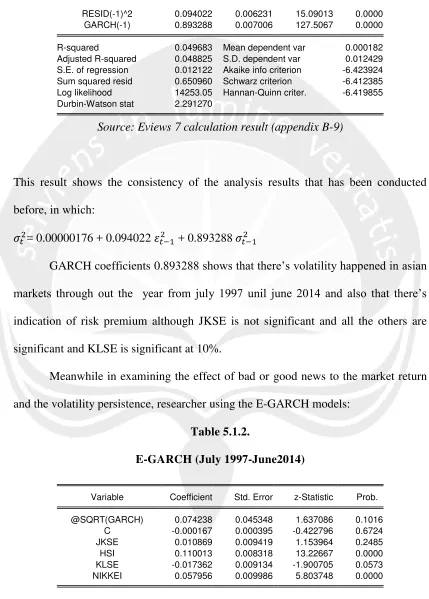
Meanwhile in examining the effect of bad or good news to the market return and the volatility persistence, researcher using the E-GARCH models:

Table 5.1.2.

E-GARCH (July 1997-June2014)

Variable Coefficient Std. Error z-Statistic Prob.

(3)

Variance Equation

C 1.70E-06 2.36E-07 7.202256 0.0000 RESID(-1)^2 0.094307 0.006259 15.06637 0.0000 GARCH(-1) 0.892987 0.007053 126.6037 0.0000

R-squared 0.047862 Mean dependent var 0.000182 Adjusted R-squared 0.046787 S.D. dependent var 0.012429 S.E. of regression 0.012135 Akaike info criterion -6.424062 Sum squared resid 0.652207 Schwarz criterion -6.411080 Log likelihood 14254.36 Hannan-Quinn criter. -6.419484 Durbin-Watson stat 2.283795

Source: Eviews 7 calculation result (appendix C-9)

This result shows the consistency of the analysis results that has been conducted before, in which:

= 0.00000176 + 0.094307 + 0.892987

Based on the results above, the information asymmetry 0.094307 which the result is positive, it means that the positive shocks cause higher volatility compared to negative shocks, this result is unanticipated and differ from what expected as written in the hypothesis, but then this study only focus on several countries in Asian, through analysis need to be conducted.

5.2. Research Limitation and Suggestion

5.3.1 Research Limitation

(4)

1. Limitation in the object of study, this study only includes the volatility, risk premia and information asymmetry as the scope of investigation, there are many other variables that actually could be examined for example the economic condition of the country, polical condition,etc. Other varibles also could be included to give better understanding about the topic and how it effect one another.

2. The number of samples for this study is limited, in which only includes of 4 country in asian and US.

3. Length of research period, is limited because of the availability of data and also time constrain. This study only able to includes 8th period in the research from 1997-2014, considering the topic which is about the volatility, the needs of the length of research period is one of the important issue that need to be highlight.

5.3.2 Suggestion

For further research, there are several points that can be suggested

1. It would be more representative if the research object is wider, added more country and not limited into Asian countries and also more samples to differ between the developed and developing countries.

(5)

3. Analyse and added more variables that need to be taken into consideration, for example the IT revolution, behavioral responses, etc.

5.3. Research Contribution

This research that has been conducted gives some insights and contribution to some aspects, there are:

5.3.1 Academic Contribution

Readers can understand the impact of volatility to the stock return, and give understanding the condition of market in several global economic events and how it

gives impact to the stock price return. Hope there‟s any future research that will be

conducted and this research give benefits to the academic activity.

5.3.2 Managerial Contribution

This research can help financial analyst who invest in Asian markets and give them understanding about the condition of the market during crisis, behavior of the stock return, and the risk of the market to help the analyst in making their international portfolio.

5.3.3 Contribution to Investor

(6)

REFERENCES

Akram, M., Sajjad, H., Fatima, T., Mukhtar, S., & Alam, H. M. (2011). Contagious Effects of Greexe Crisis on Euro-Zone States. International Journal of Business and Social Science, 2 (12), 120-129.

Bishop, S., Fitzsimmons, M., & Officer, B. (2011). Adjusting the Market Risk Premium to Reflect the Global Financial Crisis. JASSA The Finsia Journal of Applied Finance, 1, 8-14.

Casarin, R., & Squzzoni, F. (2013). Being on the Field When the Game is Still Under Way. The Financial Press and Stock Markets in Times of Crisis. Plos ONE, 8 (7), 1-14.

Chang, C. (2003). Information Asymmetry in Emerging Stock Markets and Behavioral Implications. UMI, 1-107.

Chiang, T.C., Chen, C.W.S., & So, M.K.P. (2007). Asymmetric Return and Volatility Responses to Composite News from Stock Markets. Multinational Finance Journal, 11 (3/4), 179-210.

Djamil, A.B., Razafindrambinina, D., & Tandeans, C. (2013). The Impact of

Intellectual Capital on a Firm‟s Stock Return: Evidence from Indonesia. Journal of Business Studies Quarterly, 5 (2), 176-183.

Dobano, L. A. (2013). Emerging Economies: Stock Markets After the Financial Crisis. The Journal of American Academy of Business, Cambridge, 18 (2), 98-105.

Hall, M. (2011). Response to „Adjusting the Market Risk Premium to Reflect the

Global Financial Crisis‟. JASSA The Finsia Journal of Applied Finance, 4, 11-16. Han, Y. W. (2014). Effects of Financial Crises on the Long Memory Volatility

Dependency of Foreign Exchange Rates: The Asian Crisis vs. The Global Crisis. Journal of East Asian Economic Integration, 18 (1), 3-27.

Herwany, A., & Febrian, E. (2013). Global Stock Price Linkages around the US Financial Crisis: Evidence from Indonesia. Global Journal of Business Research, 7 (5), 35-45.

Hsu, C.P., Huang, C.W., & Ntoko, A. (2013). Does Foreign Investment Worsen the Domestic Stock Market during Financial Crisis? Evidence from Taiwan. The International Journal of Business and Finance Research, 7 (4), 1-12.

(7)

Kanaoka, M. (2012). Have the Lessons Learned from the Asian Financial Crisis Been Applied Effectively in Asian Economies. International Journal of Economics and Finance, 4 (2), 103-115.

Kassim, S.H. (2012). Evidence of Global Financial Shocks Transmission: Changing Nature of Stock Markets Integration during the 2007/2008 Financial Crisis. Journal of Economic Cooperation and Development, 33(4), 117-138.

Kenani, J.M., Purnomo, J., & Maoini, F. (2013). The Impact of the Global Financial Crisis on the Integration of the Chinese and Indonesian Stock Markets. International Journal of Economics and Finance, 5 (9), 69-81.

Kolb, R.W., & Rodriguez, R.J. (1992). Financial Management. Canada: D.C. Heath and Company.

Kravets, T., & Sytlenko, A. (2013). Wavelet analysis of the Crisis Effects in Stock Index Returns. Ekonomika, 92 (1), 78-96.

Lee, G., & Jeong, J. (2014). Global Financial Crisis and Stock Market Integration between Northeast Asia and Europe. Review of European Studies, 6 (1), 61-75. Liaw, K.T. (2004). Capital Markets. South-Western: Thomson.

Lim, C.M., & Sek, S.K. (2014). Modelling the Dynamic Relationship between U.S.‟ and Malaysia‟s Stock Market Volatility. International Journal of Trade, Economics and Finance, 5 (1), 43-47.

Lukanima, B.K., & Swaray, R. (2013). Economic Cycles and Stock Return Volatility: Evidence from the Past Two Decades. International Journal of Economics and Finance, 5 (7), 50-70.

Mankiw, N.G. (2008). Principles of Economics. Singapore: Cengage Learning. Mendonca, H.F, & Nunes, M.P.D. (2011) Public Debt and Risk Premium an Analysis

from an emerging economy. Journal of Economic Studies, 33 (2), 203-217. Michie, R,C. (2006). The Global Securities Market. Oxford University Press.

Mishra, B., & Rahman, M. (2010). Dynamics of Stock Market Return Volatility: Evidence from the Daily Data of India and Japan. The International Business & Economics Research Journal, 9 (5), 79-83.

Nam, K., Kim, S.W., & Arize, A. C., (2006). Mean Aversion of Short-Horizon Stock Returns: Asymmetry Property. Review of Quatitative Finance and Accounting, 26, 137-163.

(8)

Pretorius, A., & Beer, J. (2014) Comparing the South African Stock Market‟s Response to Two Periods of Distinct Instability – The 1997-98 East Asian and Russian Crisis and The Recent Global Financial Crisis. International Business & Economics Research Journal, 13 (3), 427-442.

Rjoub, S.A.M.A., & Azzam, H. (2012). Financial crises, stock returns and volatility in an emerging stock market: the case of Jordan. Journal of Economic Studies, 39 (2), 178-211.

Royfaizal.R.C., Lee.C., & Azali. M. (2009). ASEAN -5+3 and US Stock Markets Interdependence Before, During and After Asian Financial Crisis. International Journal of Economics and Finance, 1 (2), 45-54.

Sabri, N, R. (2004). Stock Return Volatility and Market Crisis in Emerging Economies. Review of Accounting and Finance, 3 (3), 59-83.

Sekaran, U., & Bougie, R. (2010). Research Methods for Business (5th ed.). United Kingdom: John Wiley & Sons.

Shin, J. (2005). Stock Returns and Volatility in Emerging Stock Markets. International Journal of Business and Economics, 4 (1), 31-43.

Stunda, R.A. (2014). The Role of Derivatives in the Financial Crisis and Their Impact on Security Prices. Accounting & Taxation, 6 (1), 39-50.

Sum, V. (2013). Economic Policy Uncertainty in the United States and Europe: A Cointegration Test. International Journal of Economics and Finance, 5 (2), 98-101.

Swaha, P. (1993, December). Asian Capital Markets: Has the Day of the Dragon Come yet. Corporate Finance, p. 66-68.

Takemori, S., & Wada, K. (2003). Crisis and Creative Destruction: Cases of Korean and Japanese Stock Markets. Asia-Pacific Financial Markets, 10, 301-317.

Tuan, N. A., & Linh, N. (2014). The Ongoing Public Debt Crisis in the European Union: Impacts on and Lessons for Vietnam. Geopolitics, History, and International Relations, 6 (1), 94-108

Urooj, S.F., Zafar, N., & Durrani, T.K. (2009). Finding the Stock Return Volatility: A Case od KSE-100 Index. Interdisciplinary Journal of Contemporary Research in Business, 1 (4), 65-80.

(9)

(10)

APPENDIX A-1 Periodical standard deviation of stock returns

Global Stock

Market Zones Period 1 Period 2 Period 3 Period 4 Period 5 Period 6 Period 7 Period 8

JKSE Indonesia 0.027949 0.016444 0.012034 0.020471 0.022107 0.01367 0.014083 0.010674

HSI

Hong

Kong 0.027758 0.016194 0.009411 0.025166 0.029978 0.01654 0.014022 0.009619

KLSE Malaysia 0.033259 0.012795 0.006673 0.014272 0.010907 0.024704 0.006398 0.004767

NIKKEI Japan 0.017272 0.0152 0.01128 0.017529 0.028132 0.013587 0.014192 0.013487

NYSE USA 0.011303 0.011658 0.007513 0.013476 0.028287 0.013321 0.014511 0.007648 Notes: Periods: (1) The Asian Financial Crisis, (2) The Post Asian Economic Crisis, (3) The Global Economic Boom, (4) The pre Global Financial Crisis, (5) The Global Financial Crisis, (6) The Post Crisis: Economic Recovery, (7) The Greece Debt Crisis, (8) Post Crisis Period: Greece Crisis

APPENDIX A-2 Periodical mean of stock returns

Global Stock

0.00187 0.002574 0.000518 0.000418

HSI

0.00181 0.00156 -0.00037 0.000392

KLSE Malaysia -0.00167 0.000256 0.000631

-0.00086

-0.00116 0.001533 0.000198 0.00038

NIKKEI Japan -0.00058 -0.00063 0.000584 -0.0021

-0.00151 0.001096 -0.00065 0.000898

NYSE USA 0.000583 -0.00025 0.000542

-0.00062

-0.00202 0.001436 -8.3E-05 0.000635 Notes: Periods: (1) The Asian Financial Crisis, (2) The Post Asian Economic Crisis,

(11)

APPENDIX B-1. ARCH-M 1st period (the Asian Financial Crisis) Dependent Variable: NYSE

Method: ML - ARCH (Marquardt) - Normal distribution Date: 11/05/14 Time: 08:57

Sample: 7/01/1997 3/31/1999 Included observations: 457

Convergence achieved after 21 iterations Presample variance: backcast (parameter = 0.7)

GARCH = C(6) + C(7)*RESID(-1)^2 + C(8)*GARCH(-1)

Variable Coefficient Std. Error z-Statistic Prob. C 0.001353 0.000467 2.899359 0.0037 JKSE -0.021354 0.018733 -1.139910 0.2543 HSI 0.112927 0.017297 6.528660 0.0000 KLSE -0.004820 0.019480 -0.247452 0.8046 NIKKEI 0.058432 0.027927 2.092305 0.0364

Variance Equation

C 6.12E-06 2.55E-06 2.397727 0.0165 RESID(-1)^2 0.177576 0.034965 5.078637 0.0000 GARCH(-1) 0.786265 0.038289 20.53482 0.0000 R-squared 0.044992 Mean dependent var 0.000583 Adjusted R-squared 0.036541 S.D. dependent var 0.011303 S.E. of regression 0.011095 Akaike info criterion -6.324583 Sum squared resid 0.055636 Schwarz criterion -6.252378 Log likelihood 1453.167 Hannan-Quinn criter. -6.296143 Durbin-Watson stat 2.195754

APPENDIX B-2. ARCH-M 2nd period (the post Asian Economic Crisis) Dependent Variable: NYSE

(12)

Included observations: 979

Variable Coefficient Std. Error z-Statistic Prob. C -8.34E-05 0.000338 -0.246511 0.8053 JKSE 0.002194 0.018933 0.115877 0.9077 HSI 0.045436 0.021762 2.087879 0.0368 KLSE -0.030711 0.024064 -1.276178 0.2019 NIKKEI 0.098895 0.020571 4.807550 0.0000

Variance Equation

C 4.23E-06 1.24E-06 3.408224 0.0007 RESID(-1)^2 0.094800 0.017620 5.380287 0.0000 GARCH(-1) 0.873899 0.020333 42.97951 0.0000 R-squared 0.021568 Mean dependent var -0.000249 Adjusted R-squared 0.017549 S.D. dependent var 0.011658 S.E. of regression 0.011555 Akaike info criterion -6.223765 Sum squared resid 0.130056 Schwarz criterion -6.183834 Log likelihood 3054.533 Hannan-Quinn criter. -6.208573 Durbin-Watson stat 2.008249

APPENDIX B-3. ARCH-M period 3 (the Global Economic Boom) Dependent Variable: NYSE

(13)

KLSE 0.029873 0.030751 0.971439 0.3313 NIKKEI 0.048482 0.022568 2.148284 0.0317

Variance Equation

APPENDIX B-4. ARCH-M period 4 (the pre Global Financial Crisis) Dependent Variable: NYSE

Sample (adjusted): 8/01/2007 3/14/2008 Included observations: 163 after adjustments Convergence achieved after 21 iterations Presample variance: backcast (parameter = 0.7)

Variable Coefficient Std. Error z-Statistic Prob. C -0.000648 0.001098 -0.590340 0.5550 JKSE 0.180209 0.098888 1.822361 0.0684 HSI -0.043687 0.079871 -0.546967 0.5844 KLSE -0.076717 0.089282 -0.859269 0.3902 NIKKEI 0.037066 0.076307 0.485753 0.6271

Variance Equation

(14)

Adjusted R-squared 0.013641 S.D. dependent var 0.013476 S.E. of regression 0.013384 Akaike info criterion -5.724676 Sum squared resid 0.028303 Schwarz criterion -5.572835 Log likelihood 474.5611 Hannan-Quinn criter. -5.663030 Durbin-Watson stat 2.411913

APPENDIX B-5. ARCH-M period 5 (the Global Financial Crisis) Dependent Variable: NYSE

Variable Coefficient Std. Error z-Statistic Prob. C -0.001043 0.001054 -0.989556 0.3224 JKSE 0.078549 0.068783 1.141972 0.2535 HSI 0.162973 0.058437 2.788871 0.0053 KLSE -0.031903 0.109160 -0.292257 0.7701 NIKKEI 0.014887 0.078548 0.189532 0.8497

Variance Equation

(15)

Dependent Variable: NYSE

Variable Coefficient Std. Error z-Statistic Prob. C 0.000867 0.000701 1.236099 0.2164 JKSE 0.023524 0.069043 0.340717 0.7333 HSI 0.266694 0.051864 5.142218 0.0000 KLSE -0.023157 0.020161 -1.148593 0.2507 NIKKEI -0.087098 0.061465 -1.417035 0.1565

Variance Equation

APPENDIX B-7. ARCH-M period 7 (the Greece Debt Crisis) Dependent Variable: NYSE

(16)

C 0.000406 0.000551 0.736251 0.4616 JKSE 0.095400 0.058659 1.626364 0.1039 HSI 0.235646 0.056472 4.172801 0.0000 KLSE -0.002996 0.107774 -0.027802 0.9778 NIKKEI 0.021655 0.043498 0.497829 0.6186

Variance Equation

C 1.78E-06 1.05E-06 1.694992 0.0901 RESID(-1)^2 0.095593 0.016090 5.941037 0.0000 GARCH(-1) 0.897800 0.016997 52.81970 0.0000 R-squared 0.055621 Mean dependent var -8.26E-05 Adjusted R-squared 0.046605 S.D. dependent var 0.014511 S.E. of regression 0.014169 Akaike info criterion -5.956396 Sum squared resid 0.084122 Schwarz criterion -5.879986 Log likelihood 1270.756 Hannan-Quinn criter. -5.926207 Durbin-Watson stat 2.527297

APPENDIX B-8. ARCH-M period 8 (Post Crisis Period: Greece Crisis) Dependent Variable: NYSE

Variable Coefficient Std. Error z-Statistic Prob. C 0.000621 0.000270 2.301613 0.0214 JKSE 0.046330 0.027145 1.706743 0.0879 HSI 0.155350 0.031787 4.887168 0.0000 KLSE -0.122494 0.058289 -2.101498 0.0356 NIKKEI 0.040075 0.023897 1.676975 0.0935

Variance Equation

(17)

RESID(-1)^2 0.105702 0.037161 2.844444 0.0044 GARCH(-1) 0.772912 0.075886 10.18516 0.0000 R-squared 0.067825 Mean dependent var 0.000634 Adjusted R-squared 0.062150 S.D. dependent var 0.007642 S.E. of regression 0.007401 Akaike info criterion -7.005114 Sum squared resid 0.035982 Schwarz criterion -6.950791 Log likelihood 2326.693 Hannan-Quinn criter. -6.984061 Durbin-Watson stat 2.290659

APPENDIX B-9. ARCH-M (July 1997-June 2014) Dependent Variable: NYSE

Variable Coefficient Std. Error z-Statistic Prob. C 0.000436 0.000130 3.342334 0.0008 JKSE 0.010288 0.009409 1.093451 0.2742 HSI 0.110768 0.008282 13.37411 0.0000 KLSE -0.017226 0.009128 -1.887143 0.0591 NIKKEI 0.057675 0.009989 5.773794 0.0000

Variance Equation

(18)

APPENDIX C-1. E-GARCH 1st period (the Asian Financial Crisis) Dependent Variable: NYSE

Variable Coefficient Std. Error z-Statistic Prob. @SQRT(GARCH) -9.40E-05 0.208515 -0.000451 0.9996 C 0.001353 0.001899 0.712608 0.4761 JKSE -0.021352 0.018804 -1.135537 0.2562 HSI 0.112931 0.017391 6.493809 0.0000 KLSE -0.004828 0.019508 -0.247485 0.8045 NIKKEI 0.058434 0.027932 2.092025 0.0364

Variance Equation

(19)

Variable Coefficient Std. Error z-Statistic Prob. @SQRT(GARCH) 0.321184 0.142316 2.256842 0.0240 C -0.003226 0.001427 -2.261388 0.0237 JKSE 0.006827 0.019058 0.358238 0.7202 HSI 0.040095 0.022053 1.818160 0.0690 KLSE -0.026884 0.023995 -1.120414 0.2625 NIKKEI 0.096062 0.020833 4.611017 0.0000

Variance Equation

APPENDIX C-3. E-GARCH period 3 (the Global Economic Boom) Dependent Variable: NYSE

(20)

@SQRT(GARCH) 0.143114 0.153780 0.930641 0.3520 C -0.000471 0.001054 -0.446524 0.6552 JKSE 0.008996 0.019836 0.453542 0.6502 HSI 0.099832 0.025024 3.989426 0.0001 KLSE 0.030002 0.030791 0.974356 0.3299 NIKKEI 0.048531 0.022521 2.154929 0.0312

Variance Equation

APPENDIX C-4. E-GARCH period 4 (the pre Global Financial Crisis) Dependent Variable: NYSE

Sample (adjusted): 8/01/2007 3/14/2008 Included observations: 163 after adjustments Failure to improve Likelihood after 67 iterations Presample variance: backcast (parameter = 0.7)

Variable Coefficient Std. Error z-Statistic Prob. @SQRT(GARCH) 0.434507 0.166276 2.613174 0.0090 C -0.006445 0.001854 -3.475536 0.0005 JKSE 0.158603 0.093001 1.705402 0.0881 HSI -0.089399 0.078577 -1.137733 0.2552 KLSE -0.038431 0.073925 -0.519860 0.6032 NIKKEI 0.055021 0.077813 0.707093 0.4795

(21)

C 0.000151 0.000107 1.422418 0.1549 RESID(-1)^2 -0.139932 0.039662 -3.528124 0.0004 GARCH(-1) 0.276471 0.602361 0.458979 0.6462 R-squared 0.026171 Mean dependent var -0.000620 Adjusted R-squared -0.004843 S.D. dependent var 0.013476 S.E. of regression 0.013509 Akaike info criterion -5.755179 Sum squared resid 0.028651 Schwarz criterion -5.584359 Log likelihood 478.0471 Hannan-Quinn criter. -5.685828 Durbin-Watson stat 2.358921

APPENDIX C-5. E-GARCH period 5 (the Global Financial Crisis) Dependent Variable: NYSE

Variance Equation

(22)

Log likelihood 659.4096 Hannan-Quinn criter. -4.734525 Durbin-Watson stat 2.451869

APPENDIX C-6. E-GARCH period 6 (the Post Crisis: Economic Recovery) Dependent Variable: NYSE

Variable Coefficient Std. Error z-Statistic Prob. @SQRT(GARCH) 0.324046 0.245741 1.318649 0.1873 C -0.002535 0.002760 -0.918350 0.3584 JKSE 0.036581 0.071009 0.515158 0.6064 HSI 0.269741 0.055913 4.824286 0.0000 KLSE -0.025430 0.018997 -1.338660 0.1807 NIKKEI -0.133032 0.056065 -2.372817 0.0177

Variance Equation

C 1.20E-06 2.82E-07 4.276646 0.0000 RESID(-1)^2 -0.019396 0.004745 -4.087942 0.0000 GARCH(-1) 1.004707 0.003034 331.1949 0.0000 R-squared 0.083476 Mean dependent var 0.001436 Adjusted R-squared 0.066932 S.D. dependent var 0.013321 S.E. of regression 0.012867 Akaike info criterion -5.990411 Sum squared resid 0.045860 Schwarz criterion -5.874478 Log likelihood 856.6431 Hannan-Quinn criter. -5.943926 Durbin-Watson stat 2.322446

(23)

Dependent Variable: NYSE

Variable Coefficient Std. Error z-Statistic Prob. @SQRT(GARCH) 0.045023 0.137217 0.328112 0.7428 C -2.42E-05 0.001489 -0.016230 0.9871 JKSE 0.093444 0.058230 1.604740 0.1086 HSI 0.237420 0.058031 4.091287 0.0000 KLSE -0.002959 0.108705 -0.027223 0.9783 NIKKEI 0.022431 0.043465 0.516076 0.6058

Variance Equation

C 1.79E-06 1.11E-06 1.603947 0.1087 RESID(-1)^2 0.097389 0.016841 5.782794 0.0000 GARCH(-1) 0.896221 0.017326 51.72625 0.0000 R-squared 0.054847 Mean dependent var -8.26E-05 Adjusted R-squared 0.043542 S.D. dependent var 0.014511 S.E. of regression 0.014192 Akaike info criterion -5.951950 Sum squared resid 0.083396 Schwarz criterion -5.624670 Log likelihood 1207.554 Hannan-Quinn criter. -5.653558 Durbin-Watson stat 2.459366

APPENDIX C-8. E-GARCH period 8 (Post Crisis Period: Greece Crisis) Dependent Variable: NYSE

(24)

Variance Equation

APPENDIX C-9. E-GARCH (July 1997-June2014) Dependent Variable: NYSE

(25)

Variance Equation

APPENDIX D-1. Johansen Cointegration Test Result

Date: 11/05/14 Time: 11:23

Sample (adjusted): 7/08/1997 6/30/2014 Included observations: 4430 after adjustments Trend assumption: Linear deterministic trend Series: JKSE HSI KLSE NIKKEI NYSE Lags interval (in first differences): 1 to 4 Unrestricted Cointegration Rank Test (Trace)

Hypothesized Trace 0.05

No. of CE(s) Eigenvalue Statistic Critical Value Prob.** None * 0.229489 4542.259 69.81889 1.0000 At most 1 * 0.192708 3387.350 47.85613 1.0000 At most 2 * 0.180068 2439.018 29.79707 1.0000 At most 3 * 0.172592 1559.511 15.49471 1.0000 At most 4 * 0.150049 720.2137 3.841466 0.0000 Trace test indicates 5 cointegrating eqn(s) at the 0.05 level

* denotes rejection of the hypothesis at the 0.05 level **MacKinnon-Haug-Michelis (1999) p-values

Unrestricted Cointegration Rank Test (Maximum Eigenvalue)

Hypothesized Max-Eigen 0.05

(26)

None * 0.229489 1154.909 33.87687 1.0000 At most 1 * 0.192708 948.3318 27.58434 0.0001 At most 2 * 0.180068 879.5073 21.13162 0.0001 At most 3 * 0.172592 839.2973 14.26460 0.0001 At most 4 * 0.150049 720.2137 3.841466 0.0000 Max-eigenvalue test indicates 5 cointegrating eqn(s) at the 0.05 level * denotes rejection of the hypothesis at the 0.05 level

**MacKinnon-Haug-Michelis (1999) p-values

Unrestricted Cointegrating Coefficients (normalized by b'*S11*b=I):

JKSE HSI KLSE NIKKEI NYSE

-21.10821 -84.20387 20.95034 -103.2211 252.9836 -123.6950 -4.643916 130.3595 45.14988 -30.11592 -37.51875 -18.57352 -76.01662 144.2967 58.05576 -30.28299 153.1081 0.041813 -65.37057 41.53965 -66.40164 74.89552 -93.77202 -58.63086 -38.74057

Unrestricted Adjustment Coefficients (alpha):

D(JKSE) 0.003163 0.004299 0.002495 -0.000487 0.004292 D(HSI) 0.004898 -8.01E-05 -4.12E-05 -0.005514 0.001092 D(KLSE) 0.000601 -0.004401 0.002845 -0.000950 0.003753 D(NIKKEI) 0.004654 -0.001072 -0.003813 0.000477 0.002470 D(NYSE) -0.002808 0.000947 -0.002958 -0.003023 0.002616

1 Cointegrating Equation(s):

Log

likelihood 62359.92

Normalized cointegrating coefficients (standard error in parentheses)

1.000000 3.989154 -0.992521 4.890094 -11.98508 (0.24318) (0.22460) (0.26423) (0.34896) Adjustment coefficients (standard error in parentheses)

(27)

(0.00517)

1.000000 0.000000 -1.054462 -0.414937 0.359650 (0.04103) (0.04927) (0.06182) 0.000000 1.000000 0.015527 1.329864 -3.094574 (0.05486) (0.06588) (0.08267) Adjustment coefficients (standard error in parentheses)

D(JKSE) -0.598578 -0.286335 (0.03104) (0.02086) D(HSI) -0.093483 -0.412050 (0.03075) (0.02067) D(KLSE) 0.531732 -0.030165 (0.02844) (0.01911) D(NIKKEI) 0.034392 -0.386946 (0.02674) (0.01797)

(28)

Adjustment coefficients (standard error in parentheses) D(JKSE) -0.692185 -0.332675 0.437076

(0.03202) (0.02111) (0.03725) D(HSI) -0.091937 -0.411285 0.095307 (0.03209) (0.02116) (0.03733) D(KLSE) 0.424999 -0.083003 -0.777411 (0.02915) (0.01922) (0.03390) D(NIKKEI) 0.177434 -0.316133 0.247543 (0.02688) (0.01772) (0.03127) D(NYSE) 0.053153 0.286967 0.289425 (0.02562) (0.01689) (0.02980)

4 Cointegrating Equation(s):

Log

likelihood 63693.49

1.000000 0.000000 0.000000 0.000000 -2.670476 (0.07820) 0.000000 1.000000 0.000000 0.000000 -0.937581 (0.03623) 0.000000 0.000000 1.000000 0.000000 -2.245686 (0.06941) 0.000000 0.000000 0.000000 1.000000 -1.595745 (0.03955) Adjustment coefficients (standard error in parentheses)