MODEL IDENTIFICATION AND CONTROLLER DESIGN FOR AN ELECTRO-PNEUMATIC ACTUATOR SYSTEM WITH DEAD ZONE COMPENSATION
1
N. H. Sunar, 1 *M. F. Rahmat, 2Zool Hilmi Ismail, 2Ahmad ‘Athif Mohd Faudzi, 3Sy Najib Sy Salim
1
Department of Control and Mechatronics Engineering, Faculty of Electrical Engineering,
Universiti Teknologi Malaysia, 81310 Skudai, Johor, Malaysia
2
Center of Artificial Intelligence and Robotic,
Universiti Teknologi Malaysia, Jalan Semarak, Kuala Lumpur, Malaysia
3
Department of Control, Instrumentation and Automation, Faculty of Electrical Engineering,
Universiti Teknikal Malaysia Melaka, Hang Tuah Jaya, 76100 Durian Tunggal, Melaka Malaysia
Emails: [email protected]
*Corresponding author: M.F. Rahmat, [email protected]
Submitted: Mar. 5, 2014 Accepted: Apr. 15, 2014 Published: June 1, 2014
Abstract- Pneumatic actuator system is inexpensive, high power to weight ratio, cleanliness and ease of
controller. The result shows that the proposed controller reduced the overshoot and steady state error of the pneumatic actuator system to no overshoot and 0.025mm respectively.
Index terms: System identification, recursive least square, ARX, dead zone compensator, pneumatic actuator.
I. INTRODUCTION
In the past few years, there are many experimental methods have been identified by using system
identification method to obtain a mathematical modeling of the pneumatic actuator system [1]. In
the late of 1900s, the least square method has been used to identify an Auto-Regressive with
External Input (ARX) model of pneumatic actuator system [2-4]. Then, the work in [5] enhanced
the model by considering the forgetting factor. The third order Auto-Regressive Moving Average
(ARMA) model has been identified as a model structure. In [6], by using a different order, a
fourth order ARMA model has been obtained. In order to avoid complexity of nonlinear of the
system, the mix reality environment has been employed to the Recursive Least Square (RLS)
method for the identification method. Recently, a Modified Recursive Least Square (MRLS)
method has been proposed [7]. The MRLS method was improved by adaptively changes the
coefficient of forgetting factor with respect to the input and output signal.
On the other hand, the design for proper controller is also important in order to achieve an
accurate position tracking of pneumatic system. For the perfect tracking controller, the basic idea
is to achieve unity transfer function from the desired trajectory to the output of the system [8].
There are several approaches have been investigated and applied to the pneumatic system such as
PID controller, pole assignment controller, sliding mode controller [9-10], adaptive controller [7,
11], back stepping controller [12-13], fuzzy [14-15] and neural network controller [16-17]. The
tuning of the PID controller parameter have been investigated and applied to the pneumatic
system. The tuning PID controller parameters approach such as Isermann’s approach [3, 18], optimal tuning based on ITAE criteria [2] and automatic nonlinear gain PID controller [19].
Another linear control technique is the pole-assignment controller. The pole-assignment
controller is a well-known technique to control linear dynamic system. A multi-rate adaptive
pole-assignment controller has been proposed and has been experimentally proven to eliminate
pole-assignment controller has been applied to a pneumatic robot. The proposed controller has
been improving the rise-time and reducing the overshoot of the step response system. The robot
also tracked the desired position with small error by using the proposed controller [21]. Next, an
adaptive self-tuning pole-assignment controller has been investigated to the pneumatic artificial
muscles [22]. In 2013, a linear active disturbance rejection controller based on the pole
assignment controller have been applied to the pneumatic servo system [23]. The results show
that the proposed controller is robust against modeling uncertainty and external disturbance.
However, in this study, an ARX model structure identified by using RLS algorithm was chosen
as the initial of the project study. Then, a pole assignment controller was developed based on the
ARX model. A dead zone compensator is added to the system to overcome the nonlinearity of the
proportional valve.
This paper is organized as follows. Section II provides the model identification of the pneumatic
system. ARX models and the RLS method are presented. The pole-assignment method is
presented in section III. Section IV described the dead zone compensation method. The
experimental setup is provided in Section V. Section VI presented the obtained results and
discussion and finally the conclusion of overall system in Section VII.
II. METHODOLOGY
a. Modeling
System identification (SI) is a method to obtain a mathematical model of the dynamic system
based on experimental data. The identification was first introduced by Zadeh [24-25]. The other
method to obtain a mathematical model is by implementing the known law of nature. It requires
the knowledge regarding the system laws of physic, which is extremely complex for a system
likes electro-pneumatic. This makes the SI advantaged compare to the derived mathematical from
known law of nature.
The least square (LS) parameter estimator is one of the most popular estimation algorithms. The
least squares estimation was first formulated by Karl Friedrich Gauss in 1975 for astronomical
recursive least square (RLS) is developed based on the batch processing algorithm using some
matrix manipulation. This method can be done at every sampling interval.
There are four steps to determine model using SI:
(1) The input and the output data
(2) The model structure
(3) The identification method
(4) The model validation
a.i Input and Output data
In order to capture the dynamic of the system, the input signal must be chosen so that the
maximum information regarding the system response is contained in the input and output data.
The sinusoidal signal is chosen with multiple frequencies as follows:
u t( )0.5cos 2
0.07t
1.5cos 2
0.1t
0.25cos 2
0.5t
(1)a.ii The model structure
In this paper, a discrete time ARX model is chosen for the model structure of the
electro-pneumatic actuator system. The discrete time system used is in the form:
y k
Bu k
A (2)
where
1 1 1 ...
a a
n n
A a z a z (3)
0 1 1 ... b b
n n
B b b z b z (4)
a.iii The identification method
RLS algorithm can estimate the parameter b0,…,bnb & a1,…,ana by first transforming (2) into a
1
0
1 ... ... a
b n a b n T a a
y k y k y k n u k u k n
b b k (5)
The regression equation in (5) is then used in the RLS algorithm. The RLS algorithm can be
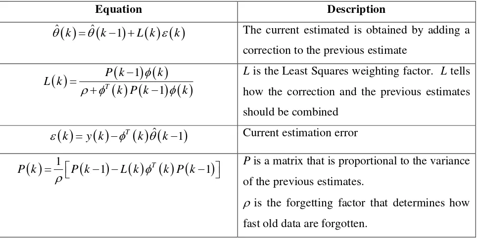
summarized as in Table 1.
Table 1: Recursive least square method algorithm
Equation Description
ˆ k ˆ k 1 L k k
The current estimated is obtained by adding a correction to the previous estimate
1
1
T
P k k
L k
k P k k
L is the Least Squares weighting factor. L tells
how the correction and the previous estimates
should be combined
T
ˆ 1
k y k k k
Current estimation error
1
1 T 1
P k P k L k k P k
P is a matrix that is proportional to the variance of the previous estimates.
is the forgetting factor that determines how
fast old data are forgotten.
a.iv The model validation
Two sets data of were taken. The first data are used for estimation process. The estimation model
then was validated with the second set of data. The best fit percentage of the estimation model
over the validation data are compare and the final prediction error is calculated. The estimated
model with highest best fit percentage and smallest final prediction error is chosen for the model
b. Pole-assignment Controller
In this research, the pole assignment controller is used to control the position tracking of the
pneumatic actuator system. The controller output used is:
u 1 Hr t
Gy t
F (6)
where:
1 1 1 ... f f
n n
F f z f z (7)
1
0 1 ...
g g
n n
Gg g z g z (8)
1
0 1 ...
h h
n n
H h h z h z (9)
The closed loop of the system is depicted in the Figure 1.
Figure 1. The closed loop of the system.
The closed loop of the system can be represented as:
k
k
z BH
y t r t
AF z BG
(10)
For pole-assignment controller, the Diophantine equation is defined as [26]:
AFz BGk T (11)
where:
1 1 1 ... t t
n n
T t z t z (12)
In order to have a unique solution for the controller coefficient, the order of F and G must follow
(1) A and B are co-prime, where A and B do not have common zeros
(2) nf nb k 1
(3) ng na1
(4) nt na nb k 1
For y(t) = r(t), at steady state, the value of H can be obtained as follow:
11
1
1
z T z H
B z
(13)
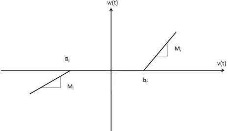
c. Dead Zone Compensator
The asymmetric dead zone was considered in this paper as in [27] and [28]. Figure 2 shows dead
zone of the valve model.
Figure 2. Dead Zone Model
The dead zone model can be represented as follow with input v(t) and output w(t):
0
r r r r
l r
l l l l
m v t m b for v t b
w t for b v t b
m v t m b for v t b
where mr, ml, br and bl are the right slope, left slope, right break point, and left break point
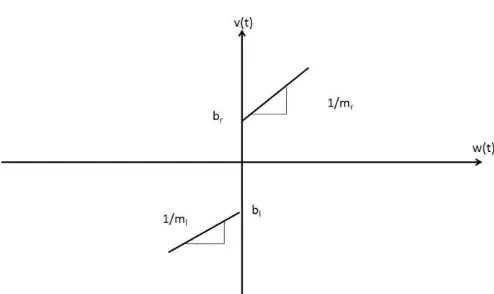
respectively. The based on the model of the dead zone, inverse dead zone model is shown in
Figure 3.
Figure 3. Inverse dead zone model
The inverse dead zone model can be write as in (15).
0
0
r r
r
l l
l
w t m b
for w t m
v t
w t m b
for w m
(15)
However, the inverse function may lead to chattering of the control input signal v(t) between the
values of bl and br when w(t) is equal to zero. For solution, a compensator as in [29-30] was
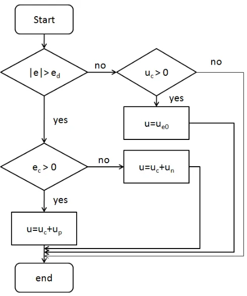
applied when w(t) is near to zero. The Figure 4, show the flow chart for the dead zone
Figure 4. Dead zone compensator flow chart
In [30], when the position error (e), exceeded the desired steady state error (ed), positive dead
zone compensation (up) and negative dead zone compensation (un) are added to the controller
output (uc) either in positive or negative direction respectively.
III. EXPERIMENTAL SETUP
a. Identification
The input used is showed in Figure 5 (a). Meanwhile, the output of the system is showed in
Figure 5(b). The input of the system is in unit voltage to the control valve: while the output of the
0 50 100 150 200 -5
0 5
(a) input
0 50 100 150 200
-200 -100 0 100 200 (b) output
Figure 5. Input and Output data of the Electro-pneumatic actuator system
A third order ARX model used in this study can be expressed as follow:
1 2
0 1 2
1 2 3
1 2 3
1
k
z b b z b z
y t r t
a z a z a z
(16)
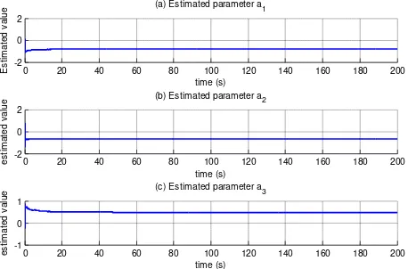
The estimated parameter a1,a2,a3 and b0,b1,b2 are shown as in Figure 4 and Figure 5 respectively.
0 20 40 60 80 100 120 140 160 180 200
-2 0 2 time (s) E s ti m a te d v a lu
e (a) Estimated parameter a1
0 20 40 60 80 100 120 140 160 180 200
-2 0 2 time (s) e s ti m a te d v a lu
e (b) Estimated parameter a2
0 20 40 60 80 100 120 140 160 180 200
-1 0 1 time (s) e s ti m a te d v a lu
e (c) Estimated parameter a3
0 20 40 60 80 100 120 140 160 180 200 -1 0 1 time (s) e s ti m a te d v a lu
e (a) Estimated parameter b0
0 20 40 60 80 100 120 140 160 180 200
-4 -2 0 time (s) e s ti m a te d v a lu
e (b) Estimated parameter b1
0 20 40 60 80 100 120 140 160 180 200
-5 0 5 time (s) e s ti m a te d v a lu
e (c) Estimated parameter b2
Figure 7. Estimated parameter b0,b1 and b2.
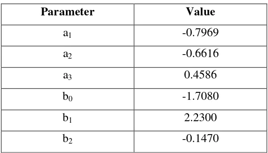
The parameter model value is shown in Table 2.
Table 2: The estimated value of the ARX model using RLS method.
Parameter Value
a1 -0.7969
a2 -0.6616
a3 0.4586
b0 -1.7080
b1 2.2300
b2 -0.1470
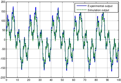
Figure 7 show the experimental output and simulation output of the electro-pneumatic actuator
system. The simulation is based on the estimated value model given in Table 2. Based on the
result, the best fit percentage between simulation and experimental output is 85.7%. The final
0 10 20 30 40 50 60 70 80 90 100 -200
-150 -100 -50 0 50 100 150 200
Experimental output Simulation output
Figure 8. Measured and Simulated Output
b. Pole-Assignment Controller
From (16), the value of na, nb and nk is 3, 2 and 1 respectively. The order of F and G can be
obtained as follow:
(1) A and B are co-prime, where A and B do not have common zeros
(2) nf nb k 1 2 1 1 2
(3) ng na 1 3 1 2
(4) nt
na nb k 1 3 2 1 1 5
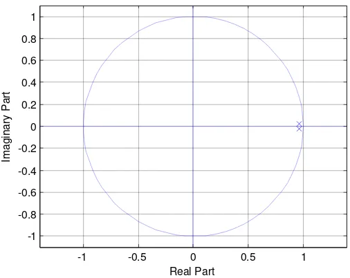
The desired pole location must be chosen in the unit circle. Figure 8 shows the desired
-1 -0.5 0 0.5 1 -1 -0.8 -0.6 -0.4 -0.2 0 0.2 0.4 0.6 0.8 1 Real Part Im a g in a ry P a rt
Figure 9. Desired characteristic equation pole location
The value of parameter F and G are solved using matrix as in (17) and H as in (13)
0 1 1 1
1 1 0 2 2 2
2 1 2 1 0 0 3
3 2 2 1 1 4
3 2 2 5
1 0 0 0
1 0
0
0 0 0
b f t a
a b b f t a
a a b b b g t
a a b b g t
a b g t
(17)
The value of parameter F, G and H are showed in Table 3.
Table 3: Obtained parameter F, G and H
Parameter Value
f1 -0.9459
f2 -0.0617
g0 0.1195
g1 -0.3090
g2 0.1925
c. Dead Zone Compensator
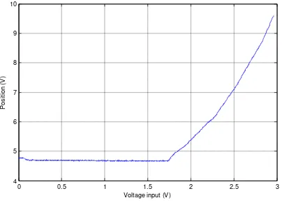
The left break point and right break point can be determined by giving a negative ramp input
voltage and positive ramp input voltage to the system. Figure 9 shows the position output in unit
voltage when given a negative ramp input voltage while Figure 10 shows the position output in
unit voltage when given a positive ramp input voltage.
-3 -2.5 -2 -1.5 -1 -0.5 0
1.5 2 2.5 3 3.5 4 4.5 5 5.5
Voltage input (v)
P
o
s
it
io
n
(
V
)
Figure 10. Position output when giving negative ramp input
0 0.5 1 1.5 2 2.5 3 4
5 6 7 8 9 10
Voltage input (V)
P
o
s
it
io
n
(
V
)
Figure 11. Position output when giving positive ramp input voltage
Table 4: Dead zone parameter value
Break point left, bl
(V)
Slope left (ml) Break point right, br
(V)
Slope right (mr)
-1.7913 2.6459 1.6713 4.4169
The un and up is 1V and 0.65V respectively.
IV. RESULTS AND DISCUSSION
a. Simulation Result Pole assignment Controller
Figure 12 shows the simulation output when giving a square input at 50mm. From the Figure 12,
the overshoot of the system is 1.99% and steady stead error is greater almost zero. The time rise
and settling time is 0.90s and 2.65s respectively.
50 52 54 56 58 60 62 64 66 68 70
-60 -40 -20 0 20 40 60
Time (s)
P
o
s
ti
ti
o
n
(
m
m
)
Input Output
Figure 12. Simulation position output when injected with square input.
The pole assignment controller with dead zone compensator was experimentally tested to the
pneumatic actuator system. Table 5 shows the comparison of the controller performance between
the simulation result of the assignment controller with experimental result of the
pole-assignment controller with dead zone compensator.
Table 5: The comparison controller performance of simulation result of pole assignment
controller with experimental result of pole-assignment controller with dead zone compensator
Control Performance Criterion
Simulation Pole assignment Controller
Hardware Pole assignment with dead zone compensator
Rise Time (s) 0.90 1.13
Settling Time (s) 2.65 1.40
Overshoot (%) 1.99 0
ess (mm) 0 0.025
c. Pole-assignment controller with dead zone compensator with varies load
The robustness of the proposed controller were tested by performing an experimental with
different payload from 0 kg to 31 kg. Figure 13 shows the position controller output with varying
50 52 54 56 58 60 62 64 66 68 70 -60
-40 -20 0 20 40 60
Time (s)
P
o
s
it
io
n
(
m
m
)
Input 0 kg 5.4 kg 10.6 kg 20.8 kg 31.0 kg
Figure 13. Position output when injected with square input with varies load
From Figure 13, as the load weight increase, the rise time and its settling time become faster. The
steady state error of the system is higher when the load weight increased. The proposed controller
results no overshoot maximum up to 31 kg. The step response characteristic can be summarized
as in Table 6.
Table 6: Step response characteristic with varies payload
Load (kg) 0 5.4 10.6 20.8 31.0
Rise Time (s) 1.13 1.12 1.10 1.10 1.13
Settling Time
(s) 1.40 1.30 1.29 1.27 1.28
Overshoot (%) 0 0 0 0 0
ess (mm) 0.025 0.15 0.52 0.21 1.09
The proposed controller was also tested to sine input for position tracking. Figure 14 shows the
50 52 54 56 58 60 62 64 66 68 70 -60
-40 -20 0 20 40 60
Time (s)
P
o
s
it
io
n
(
m
m
)
Input 0 kg 5.4 kg 10.6 kg 20.8 kg 31.0 kg
Figure 14. Position output when injected with sine input with varies load
The Figure 13 and Figure 14 shows that the proposed controller can track the given desired input.
d. Pole-assignment controller compared with Nonlinear PID
To verify with other controller method, the proposed controller was compared with the Nonlinear
PID (NPID) that was proposed in [19]. The summary of the comparison between the proposed
controller with NPID is shown in Table 7
Table 7: Comparison the performance of the pole-assignment controller with NPID controller for
the electro-pneumatic actuator system.
Pole-Assignment with dead zone compensator
NPID without dead zone compensator
Load (kg) 0 5.4 10.6 20.8 0 5.4 10.6 20.8
Overshoot (%) 0 0 0 0 0 0 5.68 5.69
The Table 7 shows that the proposed pole-assignment controller with dead zone compensator
V. CONCLUSIONS
In this study, an ARX model was identified by using an RLS method. For the position tracking
of the pneumatic actuator system, a pole-assignment controller was incorporated with dead zone
compensator. The dead zone compensation was a combination of inverse dead zone model and
the dead zone compensator to cater the steady state error. Result shows a good position tracking
performance with 0.025mm steady state error and no overshoot. The Pneumatic system was also
tested under different loads and it has been proven that the proposed controller can improved the
steady state error and the overshoot of the system. Compared with the NPID controller, the
proposed controller is robust in terms of overshoot when tested with different load. However, the
proposed controller results slower rise time and settling time. For the future work, the rise time
and the settling time can be improved to achieve the best performance of the position tracking of
the electro-pneumatic actuator system.
ACKNOWLEDGEMENT
This research is supported by the Universiti Teknologi Malaysia (UTM) and Ministry of High
Education (MOHE) through CUP grant TIER 1 vote number Q.JI30000.2523.00H36 which is
greatly appreciated. The authors are grateful for the MyPhD scholarship under the MyBrain15
program by MOHE for author scholarship.
REFERENCES
[1] M. F. Rahmat, N. H Sunar, Sy Najib Sy Salim, Mastura Shafinaz Zainal Abidin, A. A
Mohd Fauzi, and Z. H. Ismail, "Review on Modeling and Controller Design in Pneumatic
Actuator Control System," International Journal On Smart Sensing and Intelligent Systems, vol.
4, pp. pp 630-661, 2011.
[2] M.-C. Shih and S.-I. Tseng, "Identification and position control of a servo pneumatic
[3] S. Aziz and G. M. Bone, "Automatic tuning of an accurate position controller for
pneumatic actuators," in Intelligent Robots and Systems, 1998. Proceedings., 1998 IEEE/RSJ
International Conference on, 1998, pp. 1782-1788 vol.3.
[4] W.K. Lai, M.F. Rahmat, and N. A. Wahab, "Modeling and Controller Design of
Pneumatic Actuator System with Control Valve," International Journal on Smart Sensing and
Intelligent Systems, vol. 5, pp. 624-644, 2012.
[5] P. Chaewieang, K. Sirisantisamrit, and T. Thepmanee, "Pressure control of
pneumatic-pressure-load system using generalized predictive controller," in Mechatronics and Automation,
2008. ICMA 2008. IEEE International Conference on, 2008, pp. 788-791.
[6] A. Saleem, S. Abdrabbo, and T. Tutunji, "On-line identification and control of pneumatic
servo drives via a mixed-reality environment," The International Journal of Advanced
Manufacturing Technology, vol. 40, pp. 518-530, 2009.
[7] H. P. H. Anh and N. T. Nam, "Modeling and Adaptive Self-Tuning MVC Control of
PAM Manipulator Using Online Observer Optimized with Modified Genetic Algorithm,"
Engineering, vol. 3, p. 130, 2011.
[8] R. Ghazali, Y. M. Sam, M. F. Rahmat, Zulfatman, and A. W. I. M. Hashim., "Perfect
Tracking Control with Discrete LQR for a Non-minimum Phase Electro-Hydraulic Actuator
System," International Journal On Smart Sensing and Intelligent Systems, vol. 4, pp. pp 424-439,
2011.
[9] M. Taleb, A. Levant, and F. Plestan, "Twisting algorithm adaptation for control of
electropneumatic actuators," in Variable Structure Systems (VSS), 2012 12th International
Workshop on, 2012, pp. 178-183.
[10] C. Hong-Ming, C. Zi-Yi, and C. Ming-Cheng, "Implementation of an Integral Sliding
Mode Controller for a Pneumatic Cylinder Position Servo Control System," in Innovative
Computing, Information and Control (ICICIC), 2009 Fourth International Conference on, 2009,
pp. 552-555.
[11] A. Grigaitis and V. A. Gelezevicius, "Electropneumatic servo system with adaptive force
controller," in Power Electronics and Motion Control Conference, 2008. EPE-PEMC 2008. 13th,
[12] L. Chia-Hua and H. Yean-Ren, "A study on tracking position control of an pneumatic
system by backstepping design," in Control Automation Robotics & Vision (ICARCV), 2010 11th
International Conference on, 2010, pp. 721-726.
[13] M. Smaoui, X. Brun, and D. Thomasset, "A study on tracking position control of an
electropneumatic system using backstepping design," Control Engineering Practice, vol. 14, pp.
923-933, 2006.
[14] H. M. L. Eng, "Control og a Pneumatic Servosystem Using Fuzzy Logic," in Proc. of 1st
FPNI-PhD Symp. Hamburg, 2000, pp. 189-201.
[15] S. Kaitwanidvilai and P. Olranthichachat, "Robust loop shaping-fuzzy gain scheduling
control of a servo-pneumatic system using particle swarm optimization approach," Mechatronics,
2010.
[16] G. Kothapalli and M. Y. Hassan, "Design of a neural network based intelligent PI
controller for a pneumatic system," IAENG International Journal of Computer Science, vol. 35,
pp. 217-222, 2008.
[17] K. Ahn and B. Lee, "Intelligent switching control of pneumatic cylinders by learning
vector quantization neural network," Journal of Mechanical Science and Technology, vol. 19, pp.
529-539, 2005.
[18] R. B. Van Varseveld and G. M. Bone, "Accurate position control of a pneumatic actuator
using on/off solenoid valves," Mechatronics, IEEE/ASME Transactions on, vol. 2, pp. 195-204,
1997.
[19] M. Rahmat, S. N. S. Salim, N. Sunar, A. A. M. Faudzi, Z. Hilmi, and I. K. Huda,
"Identification and non-linear control strategy for industrial pneumatic actuator," International
Journal of Physical Sciences, vol. 7, pp. 2565-2579, 2012.
[20] K. Tanaka, Y. Yamada, A. Shimizu, and S. Shibata, "Multi-rate adaptive pole-placement
control for pneumatic servo system with additive external forces," in Advanced Motion Control,
1996. AMC '96-MIE. Proceedings., 1996 4th International Workshop on, 1996, pp. 213-218
vol.1.
[21] R. Richardson, M. Brown, B. Bhakta, and M. Levesley, "Impedance control for a
pneumatic robot-based around pole-placement, joint space controllers," Control Engineering
[22] A. Kyoung Kwan and A. Ho Pham Huy, "System Identification and Self-Tuning Pole
Placement Control of the Two-Axes Pneumatic Artificial Muscle Manipulator Optimized by
Genetic Algorithm," in Mechatronics and Automation, 2007. ICMA 2007. International
Conference on, 2007, pp. 2604-2609.
[23] W. Bo, W. Tao, J. Ying, F. Wei, and W. Yu, "Study of pneumatic servo system based on
linear active disturbance rejection controller," in Advanced Intelligent Mechatronics (AIM), 2013
IEEE/ASME International Conference on, 2013, pp. 1170-1174.
[24] J. Micheal, M. F. Rahmat, N. Abdul Wahab, and W. K. Lai, "Feed Forward Linear
Quadratic Controller Design for an Industrial Electro-Hydraulic Actuator System with Servo
Valve," International Journal On Smart Sensing and Intelligent Systems, vol. 6, pp. pp 154-170,
2011.
[25] C. Kaddissi, J. P. Kenne, and M. Saad, "Identification and Real-Time Control of an
Electrohydraulic Servo System Based on Nonlinear Backstepping," Mechatronics, IEEE/ASME
Transactions on, vol. 12, pp. 12-22, 2007.
[26] R. Ghazali, Y. M. Sam, M. F. Rahmat, K. Jusoff, Zulfatman, and A. W. I. M. Hashim.,
"Self-Tuning Control of an Electro-Hydraulic Actuator," International Journal On Smart Sensing
and Intelligent Systems, vol. 4, pp. pp 189-204, 2011.
[27] X.-S. Wang, C.-Y. Su, and H. Hong, "Robust adaptive control of a class of nonlinear
systems with unknown dead-zone," Automatica, vol. 40, pp. 407-413, 2004.
[28] H. Chuxiong, Y. Bin, and W. Qingfeng, "Performance-Oriented Adaptive Robust Control
of a Class of Nonlinear Systems Preceded by Unknown Dead Zone With Comparative
Experimental Results," Mechatronics, IEEE/ASME Transactions on, vol. 18, pp. 178-189, 2013.
[29] G. Sen Gupta, S. C. Mukhopadhyay, C. H. Messom, and S. N. Demidenko,
"Master–Slave Control of a Teleoperated Anthropomorphic Robotic Arm With Gripping
Force Sensing," Instrumentation and Measurement, IEEE Transactions on, vol. 55, pp.
2136-2145, 2006.
[30] Sy Najib Sy Salim, M. F. Rahmat, A. A. M. Fauzi, N. H. Sunar, Z. H. Ismail, and S. I.
Samsudin, "Tracking Performance and Distrubance Rejection of Pneumatic Actuator System," in