ISSN 1450-216X Vol.41 No.4 (2010), pp.560-569 © EuroJournals Publishing, Inc. 2010
http://www.eurojournals.com/ejsr.htm
Monetary Policy in Managing Inflation in Indonesia: A Linear
Rational Expectations Model
Iman Sugema
Department of Economics and International Center for Applied Finance and Economics Bogor Agricultural University (IPB), Bogor, Indonesia
E-mail: [email protected] Toni Bakhtiar
Department of Mathematics and International Center for Applied Finance and Economics Bogor Agricultural University (IPB), Bogor, Indonesia
E-mail: [email protected] Tel/Fax: +62 251 8348903
Abstract
This paper assesses the (in)effectiveness of monetary policy in managing inflation by employing a linear rational expectations framework. Inflation targeting is currently the main flagship of the Indonesian monetary authority and such objective is carried out within a nearly perfect open economy which is succeptible to changes in external economic situations. We consider a macroeconomic model described by a couple of structural equations which consist of several exogenous variables as shock generators. The model is then solved by implementing undetermined coefficient methods. A series of simulation based on the state space representation of the model with respect to an impulse response function is performed to highlight some of key features of current inflation trends. It is shown that monetary policies (interest rate as operating policy) can effectively affect inflation in the short run, but it has limited power in the longer run. Furthermore, its effectiveness is hampered by the so called fiscal dominance and adverse global shocks. Thus, under such a situation it would be difficult for the monetary authority to set a credible inflation target.
Keywords: Inflation targeting, open economy, rational expectation model, undetermined coefficient method.
1. Introduction
Bank Indonesia as the country’s monetary authority is by law given the task of maintaining the value of its currency. Under current policy framework, this is interpreted as inflation targeting (IT). Indeed, IT is increasingly popular amongst central bankers as the ultimate objective of monetary policy and many countries–developed and developing countries–have adopted it with great variation from lite to heavy targeting. See Bernanke et al. (1999) for lessons of inflation targeting in international perspectives.
thereby affecting the overall domestic economy. The current global crisis has greatly affected the economy–stock market plummeted by more than 50 percent, the exchange rate is among the most depreciated, and domestic commodity prices fluctuated like a roller coaster. However, despite these facts, the growth rate is sustained at 4 to 5 percent, among the highest in the world.
This paper shed lights on the difficulty of maintaining a credible inflation target during the global crisis episode. Headline inflation increased from about 6 percent to a mere 12 percent between January to May 2008, but then as global commodity prices plummeted, the inflation rate declined very rapidly to just over 2 percent. Moreover, food prices seemed to be the main driver in consumer price movements. This variation in inflation poses a question over the effectiveness of inflation targeting.
It seems clear that the current roller coaster in inflation to some extend is associated with international shocks. However, few have involved a serious rigorous modeling attempt in order to assess the impacts of the crisis on a small open economy like Indonesia. Thus, in this paper we use the most up to date modeling techniques to facilitate such assessment. We employ a dynamic open economy macroeconomic model that features rational expectations, optimizing agents, and slowly-adjusting price of goods. Pioneering publications in the area were provided by Obstfeld and Rogoff (1995, 1996). A more recent work can be found in McKibbin and Stoeckel (2009).
In this paper we develop an open economy macroeconomic model governed by a couple structural equations. Since the dynamics of the model are backward and forward looking, we adopt the so-called linear rational expectation model (LREM), which is solved by using undetermined coefficient method, to analyze the macroeconomic model. A rather comprehensive review on analyzing and solving the LREM can be found in Anderson (2006).
Based on the model we then evaluate the impacts global financial crisis and some policy measures. First, it is shown that monetary policy can in fact effectively drive inflation rate toward a certain target, at least in the short run. Second, the effectiveness of a monetary policy is hampered by a fiscal policy that moves nominal interest rate towards opposite direction which suggests the need for a coherent coordination between monetary and fiscal authorities. Third, falling international prices and global recession seem to be the dominant factor explaining the down turn in domestic inflation – rather than exchange rate depreciation.
The organization of the paper is as follows. In Section 2 we describe and solve the LREM by using undetermined coefficient method. In Section 3 we provide the considered Indonesian open economy macroeconomic model. The simulation result and discussion are in Section 4. We conclude in Section 5.
2. Linear Rational Expectation Model
The purpose of this section is to present a further explanation on formulating, solving, and analyzing linear rational expectations models by using undetermined coefficient method based on McCallum (1998).
2.1. Basic Model
Let wt be a nw × 1vector of non-predetermined endogenous variables, kt be a nk × 1vector of predetermined endogenous variables, and zt be a nz × 1vector of exogenous variables. Define the vector of endogenous variables Ωt as follow:
. t t
t w
x
⎡ ⎤ Ω = ⎢ ⎥
⎣ ⎦ (1)
The standard form of LREM under consideration is given by
1 1
, ,
t t t t
t t t
AE B Cz
z φz ε
+
−
Ω = Ω +
where Et is the expectation operator at period t, A is a square matrix of size nw + nk represents the structural coefficients matrix for future variables, B is a square matrix of the same size represent those for contemporaneous variable, εt is a nz × 1 white noise vector, and thus zt is a first-order autoregressive process whose coefficients are collected in φ.
2.2. Solution
In this part we provide the solution of (2) based on undetermined coefficient setup, where the solution is assumed in the form of:
1
, ,
t t t
t t t
w Mk Nz
k+ Pk Qz
= +
= + (3)
with M, N, P, Q are to be determined matrices. It is clear that the solution writes the non-predetermined endogenous variables as a linear combination of predetermined endogenous variables and exogenous variables.
From the second equations of (2) and (3) we have
1 ,
1 .
t t t
t t t t
E z z
E k Pk Qz
φ
+ +
=
= + (4)
By substituting into the first equation of (3) we produce
1 1 1 ( ) .
t t t t t t t t
E w+ =ME k+ +E z+ =MPk + MQ+Nφ z (5)
Hence,
1 1
1
: t t .
t t t t
t t
E w MP MQ N
E k z
E k P Q
φ
+ +
+
+
⎡ ⎤ ⎡ ⎤ ⎡ ⎤
Ω =⎢ ⎥ ⎢= ⎥ +⎢ ⎥
⎣ ⎦ ⎣ ⎦
⎣ ⎦ (6)
Together with the fact that
, 0
t
t t t t t t
t
w M N
Bw Cz B Cz B k z Cz
k I
⎛ ⎞
⎡ ⎤ ⎡ ⎤ ⎡ ⎤
+ = ⎢ ⎥+ = ⎜⎢ ⎥ +⎢ ⎥ ⎟+
⎣ ⎦ ⎣ ⎦
⎣ ⎦ ⎝ ⎠
the basic model (3) can then be written as
. 0
t t t t
M MQ N M N
A k A z B k B C z
P Q I
φ
+ ⎛ ⎞
⎡ ⎤ + ⎡ ⎤ = ⎡ ⎤ + ⎡ ⎤+
⎜ ⎟
⎢ ⎥ ⎢ ⎥ ⎢ ⎥ ⎢ ⎥
⎣ ⎦ ⎣ ⎦ ⎣ ⎦ ⎝ ⎣ ⎦ ⎠ (7)
Next we provide the solution of the model, or in other words, we explicitly determine matrices
M, N, P, Q. From (7) it is obvious that the following equalities should be satisfied: .
0
MP M MQ N N
A B A B C
P I Q
φ +
⎡ ⎤= ⎡ ⎤⇔ ⎡ ⎤= ⎡ ⎤+
⎢ ⎥ ⎢ ⎥ ⎢ ⎥ ⎢ ⎥
⎣ ⎦ ⎣ ⎦ ⎣ ⎦ ⎣ ⎦ (8)
Since the square matrices A and B may be singular, the first equality of (8) can be treated as a generalized eigenvalue problem. The generalized Schur decomposition (or qZ-decomposition) then guarantees the existence of unitary matrices q and Z, i.e., q*q = I and Z*Z = I, such that
, ,
qAZ =S qBZ =T (9)
where S and T are triangular. If S:= [sij] and T:= [tij] then the ratios λi:= tii/sii are the generalized eigenvalues of the pencil matrix B−λA. It is known that we can always arranged the eigenvalues λi and associated columns of Q and Z descendently in order of their moduli. Premultiply the first equality of (8) by q and consider the fact that qA = SZ-1 and qB = TZ-1 then we have
,
MP M
SH TH
P I
⎡ ⎤= ⎡ ⎤
⎢ ⎥ ⎢ ⎥
⎣ ⎦ ⎣ ⎦
where H = Z-1. By partitioning S, T, dan H we can write
11 11 12 11 11 12
21 22 21 22 21 22 21 22
0
0
S
H
H
MP
T
H
H
M
S
S
H
H
P
T
T
H
H
I
⎡
⎤⎡
⎤
⎡ ⎤
⎡
⎤⎡
⎤
⎡ ⎤
=
⎢
⎥⎢
⎥
⎢ ⎥
⎢
⎥⎢
⎥
⎢ ⎥
⎣ ⎦
⎣ ⎦
where the first row can be written as
(
)
(
)
11 11 12 11 11 12 .
S H M +H P=T H M +H
The above equality is satisfied only if H11M + H12 = 0. Hence, we obtain
1 11 12.
M = −H H−
Since H = Z-1, i.e.,
11 12 11 12 21 22 21 22
0 , 0
H H Z Z I
H H Z Z I
⎡ ⎤ ⎡ ⎤ ⎡ ⎤
=
⎢ ⎥ ⎢ ⎥ ⎢ ⎥
⎣ ⎦
⎣ ⎦ ⎣ ⎦ (11)
we have H11Z12 + H12Z22 = 0 or 12 11 12 221
−
= −
H H Z Z . Thus,
1 12 22.
M =Z Z− (12)
Now, the second row of (10) provides
(
)
(
)
(
)
(
)
21 11 12 22 21 22 21 11 12 22 21 22 .
S H M +H P+S H M+H P=T H M +H +T H M +H
And further
(
)
(
)
22 21 22 22 21 22 .
S H M +H P=T H M +H
The last equation holds since H11M + H12 = 0 from the first row case. Again, from (11) we have
21 12 22 22
H Z +H Z =I or H22=Z22−1−H Z Z21 12 22−1. Together with (12) we then obtain
1 1
22 22 22 22
S Z P− =T Z−
or, equivalently
1 1 22 22 22 22.
P=Z S T Z− − (13)
So far we have already identified M and P. From now we will discover N and Q. Recall the second equation of (8). By application of the generalized Schur decomposition as before we can process such that
, 0
, 0
MQ N N
qA qB qC
Q
MQ N N
SH TH D
Q φ
φ +
⎡ ⎤ ⎡ ⎤
= +
⎢ ⎥ ⎢ ⎥
⎣ ⎦ ⎣ ⎦
+
⎡ ⎤= ⎡ ⎤+
⎢ ⎥ ⎢ ⎥
⎣ ⎦ ⎣ ⎦
(14)
where we define D:= qC. Furthermore, equality in the first row can be expressed in term of the partition matrices as follows:
1 1 1 1
11 11 11 11 11 11 1.
N−H T S H N− − φ= −H T D− −
By denoting G:= −H T S H11−1 11−1 11 11 and F:= −H T D11−1 11−1 1, the last equation can be written as ,
N+GNφ=F
which can then be transformed into standard linear equation as follows:
(
I+φT⊗G)
vec( )
N =vec( )
F ,where vec(⋅) denotes vectorizations by columns of a matrix and denotes the Kronecker product. And furthermore
(
)
1vec( )N = I+φT ⊗G − vec( ).F (15)
Matrix N therefore can be obtained by inverting the vec(⋅). Next, the second row of (14)
provides
(
)
(
)
(
)
22 21 22 21 11 22 21 21 11 22 21 2.
S H M +H Q+ S H +S H Nφ = T H +T H N+D
The solution of Q then is given by
(
)
1
1 3 2 ,
Q=K− K −K (16)
where
(
)
(
)
(
)
1: 22 21 22 , 2: 21 11 22 21 , 3: 21 11 22 21 2.
3. Macroeconomic Structural Equations
In this section we provide the structural equations of Indonesian macroeconomics system considered as an open-economy model, where some external factors related to the economic transactions such as export and import, are taken into account, see McCallum and Nelson (2001). The equations are then formulated into standard linear rational expectations models and solved by undetermined coefficient method.
Most of the variables involve in the model are presented in log-linearized form. Formally, let Vt be the vector of variables and V their steady-state, then the vector of log-deviations of Vt is defined as
: log log .
t t
v = V − V (17)
In the next part we describe the structural equations, endogenous and exogenous variables which involve in the model.
3.1. Structural Equations
There are thirteen equations considered in the model. 1. Output gap
. t t t
y% = y −y (18)
Output gap y%t is the deviation between actual output yt and potential output yt. 2. Potential output
. y t t t
y =γq +e (19)
Potential output is influenced by the competitiveness (reflected by the real exchange rate qt) and the technological shock ety.
3. Price
1.
t t t
p = Δ +p p− (20)
We follow the common definition about the inflation rate Δpt, i.e., the difference of the price in the current and last periods.
4. Real exchange rate . q t t t t
q = −s p +e (21)
Here, st is the nominal exchange rate and the shock process etq constitutes the law of one price under normalized international price.
5. Uncovered interest parity (UIP)
1 ,
s t t t t t
R =E s+ − +s e (22)
where Rt is the nominal interest rate and the shock process
s t
e reflects the premium risk premium with non-constant variance and possibly inter-correlated.
6. Real interest rate
1 1.
t Rt Et t E pt t
λ = + λ+ − Δ + (23)
7. Consumption-saving
1 1 2 1 1 (1 ) .
c
t t t t t t
B E c B c B c h e
β + = − − − − β λ + (24)
The coefficients involve in this equation are the discount factors. The shock process etc
describes the stochastic shock relates to the household preferences on the current and forthcoming consumption level ct and ct+1. The forthcoming consumption depends on the real interest rate. Or, in other words, the intertemporal substitution factor is considered as an indicator which affects the consumption level.
8. Export
2 1 .
x
t t t t
The export level is given by xt. The coefficients b1 and b2 are, respectively, the substitution elasticity coefficients between real exchange rate qt and international output
*
t
y , which are exogenously considered.
9. Net export
3 ( 4 1) .
t t t t
x% = −x b y + b − q (26)
The net export level is given by x%t. Here, b4−1 can be seen as the substitution elasticity coefficient between goods and labors in the production processes.
10.Aggregate supply (AS)
(
)
1
1 1
2 .
p
t t t t t t
p αy p− E p+ e
Δ = % + Δ + Δ + (27)
The aggregate supply equation follows that of Fuhrer-Moore, where the current inflation rate is determined by the average of the last rate and the expectation for the next period. The shock process p
t
e
is assumed to have zero mean and constant variance. 11.Aggregate expenditure
1 2 3 .
t t t t
y =ηc +η x +η g (28)
The aggregate expenditure exhibits the simplification of yt =η1ct+η2xt+η3gt +η4It, where It denotes the invest level. By the equation, it does not mean that invest and import are excluded from the model. Note that the invest has been taken into account in the consumption-saving equation (24), where h denotes the elasticity coefficient between invest level and the real interest rate. Furthermore, the import is exclusively considered as the material input to the production of home-country goods, since most of the import consists of capital and material goods.
12.Monetary policy (MP) rule
1
3 1 1 4 2 3 1 3 1 4 3 1
(1 )(1 ) (1 ) (1 ) R.
t t t t t t t t t
R = −μ +μ E−Δ +p μ −μ E y− % +μR− +μ −μ E−ψ +e (29) The monetary authority is assumed obey the above equation in launching a monetary policy,
where the nominal interest rate in the current period influenced by the backward expectation of the inflation rate and the output gap.
13.Weight on inflation rate and output
1.
t pt yt yt
ψ = Δ + − − (30)
The above open-economy macroeconomics model involves 24 endogenous variables and 9 exogenous variables. Endogenous variables consist of non-predetermined (14 variables):
1
, , , , , , , , ,
, , , , .
t t t t t t t t t
t t t t t t
y y y R q s c x
p p E p x
λ
ψ Δ Δ +
%
%
and predetermined (10 variables):
1 1 1 1 1 1 1
1 1 1 1
, , , , , , ,
, , .
t t t t t t t t t t
t t t t t
c R y E E y E y p
p E p E p
ψ
− − − − − − −
− − + −
Δ
Δ Δ
%
Exogenous variables consist of government expenditure, international output, and all the shocks:
, , , , , , , , .
q y c R s p x
t t t t t t t t t
e e e e e y∗ e g e
3.2. State Space Representation
In general, the state space representation of a model is expressed as follows:
1 ,
,
t t t
t t t
X X U
Y X U
+ = Λ + Φ
= Γ + Π (31)
where Xtis the system state, Ut is the system input, Yt is the system output, and Λ, Φ, Γ, Π are the system matrices.
[
]
1
1 1
0 , 0
,
t t
t
t t
t t
t
k P Q k
e
z z I
k
w M N
z φ
+
+ +
⎡ ⎤ ⎡ ⎤⎡ ⎤ ⎡ ⎤
= +
⎢ ⎥ ⎢ ⎥⎢ ⎥ ⎢ ⎥
⎣ ⎦ ⎣ ⎦
⎣ ⎦ ⎣ ⎦
⎡ ⎤
= ⎢ ⎥
⎣ ⎦
(32)
where
[
]
10
: , : , : , : , : 0, : , : ,
0 t
t t t t t
t
k P Q
X M N U e Y w
z φ I +
⎡ ⎤ ⎡ ⎤ ⎡ ⎤
=⎢ ⎥ Λ =⎢ ⎥ Φ =⎢ ⎥ Γ = Π = = =
⎣ ⎦ ⎣ ⎦
⎣ ⎦
with the matrices are assumed having compatible dimensions.
4. Result and Discussion
In this section we provide the simulation result based on the impulse response function (IRF) approach. Here, we employ a slightly different IRF than that used in the vector autoregression (VAR) based model. While in the later model, shock is defined as one standard deviation of the variable, in the linear rational expectation framework shock refers to one unit (usually one percent) change of the variable as describe in Table 1.
Table 1: Definition of the shocks
Variable Shock Notation Definition
Technology ety Productivity increases as 1% of GDP
Government expenditure gt Primary deficit increases as 1% of the government expenditure (not from GDP)
Consumption etc Private consumption increases 1% Export competitiveness etx Export volume increases 1% International price Exogenous 1% increase
Inflation etp Exogenous inflation increases 1%
Nominal interest rate etR Domestic interest rate increases 100 points
International output yt* International output increases 1%
Figure 1: Responses of output (left), inflation (center) and nominal interest rate (right) to a monetary
tightening
0 2 4 6 8 10 12 14 16 18 20 -0.25
-0.2 -0.15 -0.1 -0.05 0
t Shock = 4, Response = 1
0 2 4 6 8 10 12 14 16 18 20 -0.4
-0.35 -0.3 -0.25 -0.2 -0.15 -0.1 -0.05 0 0.05
t Shock = 4, Response = 3
0 2 4 6 8 10 12 14 16 18 20 -0.2
0 0.2 0.4 0.6 0.8 1 1.2
t Shock = 4, Response = 4
the policy is only effective in the short run. Note that, in 2009 Bank Indonesia pursues a relatively lax policy and can be viewed as inflationary.
Figure 2: Responses of output (left), inflation (center) and nominal interest rate (right) to a fiscal expansion
0 2 4 6 8 10 12 14 16 18 20 0
0.01 0.02 0.03 0.04 0.05 0.06
t Shock = 8, Response = 1
0 2 4 6 8 10 12 14 16 18 20 0
0.005 0.01 0.015 0.02 0.025 0.03 0.035
t Shock = 8, Response = 3
0 2 4 6 8 10 12 14 16 18 20 -2
0 2 4 6 8 10 12 14 16x 10
-3
t Shock = 8, Response = 4
For the second question we simulate the effect of a 1 percent increase in budget deficit (not as percentage of GDP) which reflect the current fiscal stance (Figure 2). Such increase can boost output and inflation, but at the same time create a hike on nominal interest rate. In terms of inflation as the ultimate objective, such policy has the same result as expansionary monetary policy. However, since it increases nominal interest rate (the opposite of lax monetary policy), it tends to jeopardize the effectiveness of monetary policy. If the fiscal shock is sufficiently large, it will dominates the effect of monetary policy. This may partly explain the current difficulty lowering market interest rate. In 2009, Bank Indonesia tries to cut the policy rate but market rates stubornly not responding. Note that, medium term note (MTN) and sukuk rates are well above the Bank Indonesia rate making the market rate difficult to cut. Thus fiscal dominance is actually observed.
The third issue is how we can explain the current sliding of domestic inflation? As mentioned above both monetary and fiscal policy are inflationary, but why we have inflation rate that is lowest in six years. According to the law of one price, we have two candidates; falling international price and stronger nominal exchange rate. In addition, global recession which results in a fall in export demand may compress domestic price. Here are the simulation results.
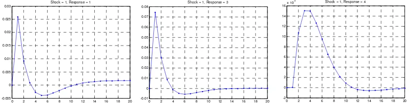
Figure 3: Responses of output (left), inflation (center) and nominal interest rate (right) to a hike in
international prices
0 2 4 6 8 10 12 14 16 18 20 -0.005
0 0.005 0.01 0.015 0.02 0.025 0.03
t Shock = 1, Response = 1
0 2 4 6 8 10 12 14 16 18 20 -0.01
0 0.01 0.02 0.03 0.04 0.05 0.06 0.07 0.08
t Shock = 1, Response = 3
0 2 4 6 8 10 12 14 16 18 20 -2
0 2 4 6 8 10 12 14 16x 10
-3
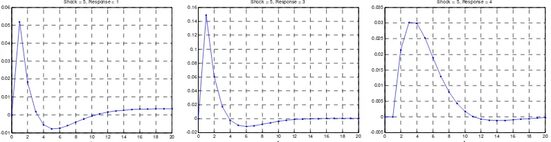
Figure 4: Responses of output (left), inflation (center) and nominal interest rate (right) to nominal exchange rate depreciation
0 2 4 6 8 10 12 14 16 18 20 -0.01
0 0.01 0.02 0.03 0.04 0.05 0.06
t S hock = 5, Response = 1
0 2 4 6 8 10 12 14 16 18 20 -0.02
0 0.02 0.04 0.06 0.08 0.1 0.12 0.14 0.16
t Shock = 5, Response = 3
0 2 4 6 8 10 12 14 16 18 20 -0.005
0 0.005 0.01 0.015 0.02 0.025 0.03 0.035
t Shock = 5, Response = 4
Figure 5: Responses of output (left), inflation (center) and nominal interest rate (right) to an increase in global
output
0 2 4 6 8 10 12 14 16 18 20 -0.15
-0.1 -0.05 0 0.05 0.1 0.15 0.2 0.25 0.3 0.35
t S hock = 6, Response = 1
0 2 4 6 8 10 12 14 16 18 20 -0.4
-0.3 -0.2 -0.1 0 0.1 0.2 0.3
t Shock = 6, Response = 3
0 2 4 6 8 10 12 14 16 18 20 -0.05
0 0.05 0.1 0.15 0.2 0.25 0.3 0.35
t Shock = 6, Response = 4
Figure 3 suggests that an increase in international price tends to increase output, interest rate and inflation rate. As we already know, since mid 2008 international commodity prices droped dramatically until mid 2009. Thus the fall in commodity price is a likely candidate for explaining the low inflation. If this is true, then we can expect that in 2010 inflation will increase as commodity price is currently on the upswing trend. Figure 4 suggests that a nominal exchange rate depreciation tend to have an expansionary effect on output, inflation and interest rate. Thus, because the rupiah depreciated in October 2008 and gradually strengthening lately, such exchange rate movement is not the likely candidate for explaining low inflation. Figure 5 suggests that an increase in international output tend to increase domestic output (via export), interest rate and inflation rate. Thus, a global economic crisis will tend to reduce domestic output and press down interest rate and inflation. This is consistent with factual situation.
In summary, the low inflation rate is not the result of monetary as well as fiscal policies. Moreover, exchange rate movement has little to say about low inflation. It is likely that the fall in international prices and output are the factors.
5. Conclusion
In this paper we have developed a theoretical dynamic stochastic general equilibrium (DSGE) model for Indonesia. An open-economy with forward looking agents has been adopted and connections to international market are incorporated.
References
[1] B. S. Bernanke, T. Laubach, F.S. Mishkin and A.S. Posen, 1999, “Inflation Targeting: Lessons from International Experience,” Princeton University Press.
[2] M. Obstfeld and K. Rogoff, 1995, “Exchange Rate Dynamics Redux,” Journal of Political Economy, 103, 624–660.
[3] M. Obstfeld and K. Rogoff, 1996, “Foundations of International Macroeconomics,” Cambridge MA: MIT Press.
[4] W.J. McKibbin and A. Stoeckel, 2009, The Global Financial Crisis: Causes and Implications,
Working Paper in International Economics, Lowy Institute.
[5] G.S. Anderson, 2006, “Solving Linear Rational Expectations Models: a Horse Race,” Manuscript, Finance and Economics Discussion Series, Federal Reserve Board.
[6] P. Klein, 2000, "Using the Generalized Schur Form to Solve a Multivariate Linear Rational Expectation Model. Journal of Economic Dynamics and Control, 24(10), 1405–1423.
[7] B.T. McCallum, 1998, “Solutions to Linear Rational Expectations Models: a Compact Exposition,” Economics Letters, 61, 143–147.
[8] B.T. McCallum, 2001, “Software for RE analysis,” Manuscript.