Ordinal Logistic Regression Model and Biplot Analysis to Determine Factors Influencing Backward Region Status.

(1)

ORDINAL LOGISTIC REGRESSION MODEL AND BIPLOT ANALYSIS

TO DETERMINE FACTORS INFLUENCING

BACKWARD REGION STATUS

NOVERA ELBA RORA

DEPARTMENT OF STATISTICS

FACULTY OF MATHEMATICS AND NATURAL SCIENCES

BOGOR AGRICULTURAL UNIVERSITY

(2)

ABSTRACT

NOVERA ELBA RORA.Ordinal Logistic Regression Model and Biplot Analysis to Determine Factors Influencing Backward Region Status. Under the supervision of ASEP SAEFUDDIN and DIAN KUSUMANINGRUM.

The functions of State Ministry of Acceleration of Development in Backwards Regions are to formulate national policy in the field of development in backwards region sector, to implement the policy, to organize stated-owned properties or assets, to supervise the implementation of its duty, to submit the evaluation report, suggestion and consideration in its assignment and function to the President. In order to reach these objectives, the government needs to understand the prior concern so development will be effective and efficient. Therefore, it is important to analyze the relevant factors that influence the backward region status. The objective of this research were to determine factors influencing the backward region status to provide good policy and appropriate allocation of assets or fund. Ordinal logistic regression and biplot were used to analyze the status of backward regions with 33 explanatory variables. The explanatory variables identified as significant factors were the percentage of poor people, poverty index, the percentage of malnutrition children under five, live expectancy, the percentage of access to health infrastructure, average number of drop out elementary school students, the percentage of family using electricity, the percentage of rural areas without nonpermanent market, average distance between “kantor desa”(village office) and “kantor kabupaten”(district office), and the percentage of rural areas with critical land. To analyze the regional disparity (between east and west), biplot was implemented and the variables were clustered according to the regional differences.

(3)

ORDINAL LOGISTIC REGRESSION MODEL AND BIPLOT ANALYSIS

TO DETERMINE FACTORS INFLUENCING

By:

NOVERA ELBA RORA

G14104005

Thesis

For the partial fulfillment for the degree of Bachelor of Sciences

Faculty of Mathematics and Natural Sciences

Bogor Agricultural University

DEPARTMENT OF STATISTICS

FACULTY OF MATHEMATICS AND NATURAL SCIENCES

BOGOR AGRICULTURAL UNIVERSITY

(4)

Title

: ORDINAL LOGISTIC REGRESSION AND BIPLOT

ANALYSIS TO DETERMINE FACTORS INFLUENCING

Name

: Novera Elba Rora

NRP

: G14104005

Approved by:

Advisor I,

Dr. Ir. Asep Saefuddin, M.Sc

NIP. 130938261

Advisor II,

Dian Kusumaningrum, S.Si

Acknowledged by:

Dean of Faculty of Mathematics and Natural Sciences

Bogor Agricultural University

Dr. drh. Hasim, DEA.

NIP. 131578806

(5)

BIOGRAPHY

(6)

ACKNOWLEDGEMENT

Alhamdulillahi rabbil ‘alamin, praise and grateful to Allah SWT for all blessing and favour that made this thesis which is entitled “Ordinal Logistic Regression Model and Biplot Analysis to Determine Factors Influencing Backward Region Status” completed.

This thesis could not been written without the support from many people, therefore, in this opportunity, the author would like to acknowledge the following people :

1. Dr. Ir. Asep Saefuddin, M.Sc. and Dian Kusumaningrum, S.Si for the valuable advice, theoretical guidance, supports, and critics during this research. They were my main adviser.

2. All lecturers at Department of Statistics for sharing their knowledge and also staffs of Department of Statistics for helping my study: Bu Aat, Bu Markonah, Bu Sulis, Bang Sudin, Pak Ian, Mang Herman, and Bang Dur.

3. My beloved family mama, papa, Adek Ica and Adek Chairul for all prayer, supports, love, and advices.

4. For Tiga Diva (Yuyun K and Ratih Noko), Empat Sahabat (Nidia, Yuyun, Riski), Pandawa Lima, Listya, and Nurhasanah thanks for togetherness to understand the essence of struggling.

5. For all STK’41: Wiwik, Wita, Rere, Yusri, Wenny, Rizqa, Ika, Ami, Cheri, Ratih Nurma, Irene, Sevrien, Tjipto, Ihsan, Ikin, Doddy, Inal, Rangga, Efril, Coy, Heri (thanks for all your support), Vinda my partner at ICCRI, and others who can not be mentioned here, I am very thankful for the friendship and the times that we had together.

6. All STK’40, STK’42 (especially Indah and Dewi as my panelist), STK’43 and STK’44. 7. All my friend in Andaleb 2, my beloved boarding house.

8. All of Light Blue and 4S team for your advises, never give up to spread the light. 9. BeST team (thanks for your support).

And many others who could not be mentioned one by one in this opportunity. Thank you for everything. The author realized that perfection only belongs to Allah SWT and that there is still a lot of lack in this thesis. Hopefully, this thesis is useful for everybody especially government and somebody who needs the information in this thesis.

Bogor, January 2009

(7)

LIST OF TABLES

Page

1. Name of regencies that are outliers ... 4

2. Variables with strong correlation ... 4

3. Value of significant estimation parameter of Economic criteria ... 4

4. Value of significant estimation parameter of Human Resources criteria ... 5

5. Value of significant estimation parameter of Infrastructure criteria ... 5

6. Value of significant estimation parameter of Accessibility criteria ... 6

7. Value of significant estimation parameter of Characteristic of regions criteria ... 6

LIST OF FIGURES

Page 1. Number and percentage of regency with each status ... 3

2. Biplot of All Indonesian Regions ... 7

3. Biplot of Western and Eastern part of Indonesian Backward Region ... 8

LIST OF APPENDICES

Page 1. List of response variables ... 10

2. Result of Ordinal Logistic Regression of Economic Criteria ... 11

3. Result of Ordinal Logistic Regression of Human Resource Criteria... 12

4. Result of Ordinal Logistic Regression of Infrastructure Criteria ... 13

5. Result of Ordinal Logistic Regression of Region Finance Criteria ... 14

6. Result of Ordinal Logistic Regression of Accessibility Criteria ... 14

7. Result of Ordinal Logistic Regression of Characteristic Region Criteria ... 15

8. Result of Biplot analysis All Indonesian Regions ... 16

(9)

1

INTRODUCTION

Background

The central and local government have developed various programs in order to improve the welfare of society in all Indonesian regions. Centralization of development has affected large gaps among regions in and out of Java, western and eastern part of Indonesia, and between urban and rural area. There are more than 70.611 villages in Indonesia, 32.379 of them are categorized as backward region with 62% of these villages are located in the eastern regions of Indonesia (KNPDT, 2004).

The Government of Indonesia (GoI) needs to accelerate development in backward regions to overcome the problems. The fundamental purpose of accelerating development in backward regions is to empower backward society to fulfill their basic needs so they can do the activities that play a crucial role in balancing with the other societies in Indonesia. Therefore, since 2004 the government has realized the importance of developing the State Ministry of Acceleration of Development in Backward Regions (KNPDT, 2004).

The functions of State Ministry of Acceleration of Development in Backward Regions (KNPDT) are (1) to formulate national policy in the field of development in backward regions sector, (2) to implement the policy (3) to organize stated-owned properties or assets, (4) to supervise the implementation of its duty, (5) to submit the evaluation report, suggestion and consideration in its assignment and function to the President (KNPDT, 2004). In order to reach these objectives, the GoI must know which are the prior concerns so that the development will be effective and efficient.

The GoI has used 33 explanatory variables to determine backward region status. These variables are possibly correlated one to another. Therefore, it is very important to simplify factors that most influence backward region status for further analysis. Ordinal logistic regression was implemented to find the most influential factor. In addition, biplot was used to present graphically information of relationships between explanatory variables and observations.

Objective

The objectives of this research were to 1. Determine factors that strongly influence

the backward region status and give

recommendation to the GoI for making good policy and appropriate allocation of assets or fund based on these factors. 2. Present graphical information of

relationship between explanatory and observation variables. It is also interesting to compare the condition of western and eastern part of Indonesia, taking into mind that most of backward regions are located in the eastern regions of Indonesia.

LITERATURE REVIEW

Backward Regions

Backward regions are regencies in Indonesia that are relatively undeveloped compared with other regions in the country (KNPDT, 2004).

Poverty

Poverty is a deprivation of common necessities that determine the quality of life, including food, clothing, shelter and safe

drinking water, and may also include the deprivation of opportunities to learn, to obtain better employment to escape poverty, and or to enjoy the respect of fellow citizens. The

World Bank defines extreme poverty as living on less than US$ 1 per day, and moderate poverty as less than US$ 2 a day (Wikipedia, 2008).

Ordinal Logistic Regression

Logistic regression extends categorical data analysis to data sets with binary response and one or more continuous factor (Freeman 1987). Ordinal logistic regression perform logistic regression on an ordinal response variable. One way to use category ordering forms logit of cumulative probabilities for ordinal response Y with c categories, x are explanatory variables. The cumulative probability for each category can be formulated as

) ( ) |

(Y j x F x

P ≤ = _j

=π₁(x)+...+πj(x)……….(1) where π_j(x)is the response probability of the jth category of an explanatory variable x. Cumulative logits for each category j are defined as

; wherej=1,2,...,c−1..…(2)

A model that simultaneously uses all cumulative logits can be written as

(10)

x x

Lˆ_j( )=α +ˆ_j βˆ' ………...(3) Each cumulative logit has its own intercept. The are increasing in j, since P(Y≤j|x) increases in j when x is fixed, and the logit is an increasing function of this probability (Agresti, 2002). and are the maximum likelihood estimators for each and . These estimators represent the change in logits cumulative for each j category, if the other explanatory variables do not influence

) ( ˆ _x

Lj . The interpretation of the βˆ' is the

change in logit cumulative for each j category, in other hand, odds ratio will change equal to exp (βˆ') for each change of explanatory variables x (Agresti, 2002).

The estimate value for P(Y≤j|x)can be derived with inverse transformation of logit cumulative function, the result will be shown below.         + + + = ≤ ) ' ˆ ˆ exp( 1 ) ' ˆ ˆ exp( ) | ( x x x j Y P j j β α β α _{…………..(4)}

where j=1, 2, …, c-1 or         − − + = ≤ ) ' ˆ ˆ exp( 1 1 ) | ( x x j Y P j β α ………..(5) so that         − + = ≤ )) ( ˆ exp( 1 1 ) | ( x L x j Y P j ……….(6)

Testing the Model Significance

Likelihood ratio test of the overall model is used to assess parameter

β

_iwith hypothesis : H0 : β1=...=βp=0

H1 : at least there is one

where i is the number of explanatory variables.

The likelihood-ratio test uses G statistic, which is G = -2 ln(L0/Lk) where L0 is

likelihood function without variables and Lk is

likelihood function with variables (Hosmer & Lemeshow 2000). If H0 is true, the G statistic

will follow chi-square distribution with p degree of freedom and H0 will be rejected if

value of G > X2(p,α) or p-value < α.

A Wald test is used to test the statistical significance of each coefficient β_i in the model.Hypothesis are

H0 : β_i =0

H1 : βi≠0;i=1,...,p

where i is the number of explanatory variables.

A Wald test calculates a W statistic, which is formulated as ) ˆ ( ˆ ˆ i i SE W i β β

β = ……….……….(7)

Reject null hypothesis if |W| > Zα/2 or

p-value < α(Hosmer & Lemeshow, 2000).

Assumption of Logistic Regression

Logistic regression is popular in part because it enables the researcher to overcome many of the restrictive assumptions of OLS (Ordinary Least Square) regression:

1. Logistic regression does not assume a linear relationship between the dependent and the independent variables. It can handle nonlinear effects even when exponential and polynomial terms are not explicitly added as additional independents because the logit link function on the left-hand side of the logistic regression equation is non-linear. 2. The dependent variable does not need to

be normally distributed (but does assume that its distribution is within the range of the exponential family distributions, such as normal, Poisson, binomial, gamma). Solutions may be more stable if the predictors have a multivariate normal distribution.

3. The dependent variable does not need to be homoscedastic for each level of the independents; that is, there is no homogeneity of variance assumption: variances does not need to be the same within categories.

4. Normally distributed error terms are not assumed.

5. Logistic regression does not require that the independents be an interval scale variable.

However, other assumptions still apply: 1. The data doesn’t have any outliers. As in

OLS regression, outliers can affect results significantly. The researcher should analyze standardized residuals for outliers and consider removing them or modeling them separately. One way for detecting multivariate outliers is with mahalanobis distance. Mahalanobis distance is the leverage times (n - 1), where n is the sample size. As a rule of thumb, the maximum Mahalanobis distance should not exceed the critical chi-square value with degrees of freedom equal to the number of predictors and

α = 0.001, or else outliers may be a problem in the data.

j αˆ j αˆ βˆ' j α p i

i ≠0; =1,2,..., β

'

(11)

2. Between explanatory variables there should be no multicollinearity: to the extent that one independent is a linear function of another independent, the problem of multicollinearity will occur in logistic regression, as it does in OLS regression. As the correlation among each other increase, the standard errors of the logit (effect) coefficients will become inflated. Multicollinearity does not change the estimates of the coefficients, only their reliability. High standard errors flag possible multicollinearity (www.chass.ncsu.edu).

Biplot Analysis

Biplot similarity provides plots of the n observations, but simultaneously they give plots of positions of the p variables in two dimensions. Furthermore, superimposing the two types of plots provides additional information about relationships between variables and observations not available in either individual plot (Jolliffe, 2002).

The plots are based on the singular value decomposition (SVD). This state that the (n x p) matrices X on observations on p variables measured about their sample means can be written

X = ULA׳

where U, A are (nxr),(pxr) matrices respectively, each with orthonormal columns,

L is an (rxr) diagonal matrix with elements

2 / 1 2 / 1 1 2 / 1

1

t

...

t

r

t

≥

, and r is the rank of X.

To include the information on the variables in this plot, we consider the pair of eigenvectors. These eigenvectors are the coefficient vectors for the first two sample principal components. Consequently, each row of matrix positions a variable in the graph, and the magnitudes of the coefficients (the coordinates of the variable) show the weightings that the variable has in each principal component. The positions of the variables in the plot are indicated by a vector.

MATERIAL AND METHODS Source of Data

The data used in this study were collected from the KNPDT. These data were derived from data Potensi Desa (Podes) 2005 and Survei Sosial Ekonomi nasional (Susenas) 2006 conducted by Central Bureau of Statistics (CBS). The data consists of five categories as response variable and 33

explanatory variables which can be seen in Appendix 1.

Method

The methods used in this research were: 1. Data preparation.

This step consist of selecting regencies with backward region status namely fairly backward, backward, very backward and the most backward regions.

2. Early data description.

3. The assumption of a logistic regression examination.

4. Data analysis.

Analyze selected data with ordinal logistic regression. This analysis is conducted for each sub criteria of determining backward region status.

5. Determine the prior factors that influence backward region status.

6. Significant variables were further analyzed through biplot and then explain the relationship of these variables based on globally and part of regions (west and east).

The Software used in this research are Microsoft Excel 2007, Minitab 14, SPSS 13 and SAS 9.1.

RESULTS AND DISCUSSION

Early Description

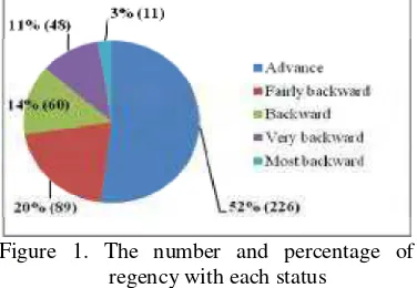
According to the data released by KNPDT, there are 434 regencies in Indonesia. KNPDT has determined five categories of region index and status based on six major criteria, such as (1) economic, (2) human resources, (3) infrastructures, (4) regional finance, (5) accessibility, and (6) characteristic of region. Each criteria has indicators which are relevant to measure the criteria score. Then the GoI calculated region score with giving weight for each criteria based on their experiences and then multiply it with standardized data.

Figure 1. The number and percentage of regency with each status

(12)

focused on backward region status. Hence, the data which were used in this research were just 208 regencies with status namely fairly backward, backward, very backward and the most backward regions. According to the minister of KNPDT, the acceleration development in backwards regions is an absolute requisite for nation advancement especially in integration sector (Karel, 2008).

Before modeling the data, there should be an examination towards the assumption of ordinal logistic regression. First, examined the multivariate outliers with mahalanobis distance. There were 11 outliers that can be seen in the table below. The outliers can be removed from the data. Hence, just 197 regencies were used in this analysis.

Table 1. Name of regencies that are outliers

Province Name of Regencies

Backward Region Status

Bengkulu Seluma Backward Jambi Batanghari Fairly

Backward Kalimantan

Barat

Bengkayang Fairly Backward Sintang Fairly

Backward Lampung Way Kanan Backward Riau Pelalawan Fairly

Backward Sulawesi

Selatan

Bulukumba Fairly Backward

Gowa Fairly

Backward

Luwu Backward

Sulawesi Bombana Backward Tenggara Kolaka Fairly

Backward

The second assumption was there should be no multicollinierity. For examining this assumption, we examine the correlation among the explanatory variables. After counting the correlation, there were strong correlation between variables, which can be seen in the table 2.

Table 2. Variables with strong correlation Variables*) Pearson Correlation

X22 and X23 0.85

X24 and X25 0.89

X28 and X29 0.85

Multicollinierity problem can be overcame by deleting one of the paired variables that were

strongly correlated. Variables that were deleted from the explanatory variables were X23 (the percentage of malnutrition people above five), X24 (infant mortality rate), and X28 (average of health infrastructure distance). Hence, there were only 30 explanatory variables used in this analysis.

Prior Factors that Influence Backward Region Status

As the result of ordinal logistic regression between Y (response variable) and each major criteria, just one major criteria which consist of 1 explanatory variable was not statistically significant. This criteria was regional finance criteria. There were just 10 from 30 explanatory variables that were statistically significant based on ordinal logistic regression.

Appendix 2 to 7 described the result of each ordinal logistic regression that has a p-value of G test less than 0.05, except for regional finance criteria. This indicated that these models provide an adequate description of the data. In the following paragraphs we can see the result of each criteria individually.

Economic Criteria

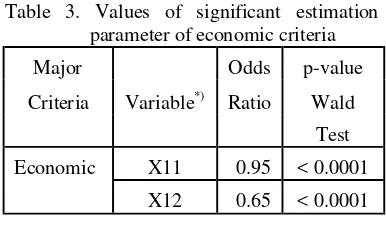
The GoI has determined two sub criterias for Economic criteria. That were the percentage of poor people and poverty index. The result of ordinal logistic regression is shown in table below.

Table 3. Values of significant estimation parameter of economic criteria

Major Odds p-value

Criteria Variable*) Ratio Wald

Test

Economic X11 0.95 < 0.0001

X12 0.65 < 0.0001

The significant explanatory variables of Economic criteria were the percentage of poor people (X11) and poverty index (X12). The cumulative logit of ordinal logistic regression model is given by the equation below.

) ( ˆ _x

L_j = constant (j) - 0.055 X11 - 0.435 X12

Values of constant (j) for j = 1,2,3 in the

(13)

regression model was similar for each major criteria. For example, in economic criteria. X11 (the percentage of poor people variable) has an estimated parameter equal to -0.055. This indicated that the estimated odds ratio for

the increasing of 1% of poor people is e-0.055= 0.95, it means that when the

percentage of poor people increases then the probabilities of becoming a backward region would definitely increase.

The most critical political-economic issue facing Indonesia is poverty reduction. Poverty in Indonesia, measured in income terms, affect 48% of Indonesia’s total population of 220 million. The government’s Medium Term Development Program aims to reduce the poverty head count from 18.2% in 2004 to roughly 8.4% by 2009 (Sudarsono, 2007). Therefore, the GoI needs to reduce the percentage of poor people and poverty index in backward region in Indonesia.

Human Resources Criteria

The GoI has determined 13 sub criterias for human resources criteria. It consists of employment, health and education sector. The result of ordinal logistic regression is shown in table below.

Table 4. Values of significant estimation parameter of human resources criteria

Major Odds p-value

Test

Human X22 0.87 < 0.0001

Resources X25 1.27 < 0.0001

X29 0.96 < 0.0001

X211 0.93 0.006

The significant explanatory variables of human resources criteria were the percentage of malnutrition children under five (X22), live expectancy (X25), the percentage of access to health infrastructure (X29), and average number of Elementary school Drop Out students (X211). The cumulative logit of ordinal logistic regression model is given by the equation below.

) ( ˆ _x

L_j = constant(j) - 0.142 X22 + 0.214 X25

- 0.041 X29 - 0.075 X211

An example of interpretation of the explanatory variable X25 (live expectancy) will be given by having an estimated parameter equal to 0.214, indicated that the estimated odds ratio for the increasing of live expectancy is e0.214= 1.27. It means that when live expectancy increase then the probabilities of becoming a backward region would definitely decrease.

Human resources criteria, one of most influential factors of backward region status that consists of health, education, and live expectancy sectors. The government has

continuously improved the Indonesian

educational system and human resources development especially in backward regions. Many programs related with these sectors should be implemented in backward regions.

Infrastructure Criteria

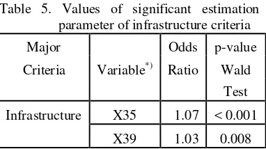
The GoI has determined 9 sub criterias for infrastructure criteria. It consists of transportation infrastructure, electricity, telephone, bank, and market sector. The result of ordinal logistic regression is shown in table below.

Table 5. Values of significant estimation parameter of infrastructure criteria

Major Odds p-value

Test

Infrastructure X35 1.07 < 0.001

X39 1.03 0.008

The significant explanatory variables of infrastructure criteria were the percentage of family using electricity (X35) and the percentage number of rural areas with nonpermanent market (X39). The cumulative logit of ordinal logistic regression model is given by the equation below.

) ( ˆ _x

Lj = constant (j) + 0.067 X35 + 0.028 X39

The government has continuously improved the infrastructure especially in backward regions. Many programs such as providing electric installation and road development should be implemented in backward regions.

(14)

Regional Finance Criteria

The GoI has defined fiscal gap as regional finance criteria. Fiscal gap was measured by substracting the region income with region expenditure. Particularly for region finance criteria, the result of ordinal logistic regression with response variable backward region status and explanatory variables of region finance criteria has a p-values 0.7 for the G test (more than 0.05). It indicated that this model doesn’t provide an adequate description of the data. Wald test reveals that the region finance criteria named fiscal gap was statistically insignificant.

Accessibility Criteria

The GoI has determined average distance between “kantor desa”(village office) and “kantor kabupaten”(district office) for accessibility criteria. The result of ordinal logistic regression is shown in table below.

Table 6. Values of significant estimation parameter of accessibility criteria

Major Odds p-value

Test

Accessibility X51 0.98 < 0.0001

The significant explanatory variables of the accessibility criteria were the average distance between “kantor desa”(village office) and “kantor kabupaten”(district office) (X51). The cumulative logit of ordinal logistic regression model is given by the equation below.

) ( ˆ _x

Lj = constant (j) – 0.024 X51

Basic infrastructure services is important to sustain economic growth and improve people’s standards of living. Accessibility and characteristic of regions also give an influence to accelerate the development of backward region status. Many programs should be implemented by the GoI to overcome the problems in infrastructure sectors in backward regions.

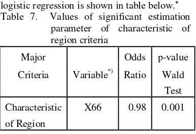
Characteristic of Region Criteria

The GoI has determined 7 sub criterias for characteristic of region criteria. It consists of rural areas earthquake, flood, landslide and

the other disasters. The result of ordinal logistic regression is shown in table below.∗ Table 7. Values of significant estimation

parameter of characteristic of region criteria

Major Odds p-value

Test

Characteristic X66 0.98 0.001

of Region

The significant explanatory variables of characteristic criteria was the percentage of rural areas with critical land (X66). The cumulative logit of ordinal logistic regression model is given by the equation below.

) ( ˆ _x

Lj

=

constant(j) – 0.023 X66

Generally, according to ordinal logistic regression, there were only five from six major criteria that influences the backward region status. It was not appropriate with the government’s criteria. The GoI must consider not to include the region finance indicator or choose another indicator for the characteristic of region criteria.

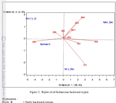
Biplot Analysis of All Indonesian Backward Regions

Figure 2 shows that the biplot represents 98.5% of the total variance in the data. First axis gives 95.6% and second axis gives 2.9% for total variance.

Biplot in figure 2 show that fairly backward regions were influenced by X25 (live expectancy) and X39 (the percentage number of rural areas without nonpermanent market). Backward regions were most influenced by X35 (the percentage of family using electricity). Very backward regions were most influenced by X11 (the percentage of poor people), X29 (the percentage of access to health infrastructure), and X51 (average distance between “kantor desa” (village office) and “kantor kabupaten” (district office)). Most backward regions were most influenced by X12 (poverty index), X22 (the percentage of malnutrition children under five), X211 (average number of Elementary school Drop Out students), and X66 (the percentage of rural areas with critical land).

*

(15)

7

Figure 2. Biplot of all Indonesian backward region

Explanation :

Fairly_B = Fairly backward regions Backward = Backward regions Very_Bac = Very backward regions Most_Bac = Most backward regions

According to the biplot analysis, many programs related with these sectors should be implemented in each backward region’s category. The GoI should consider many programs that related with these

significant explanatory variables as first

priority of development.

Biplot Analysis of Western and Eastern part of Indonesian Backward Regions

According to KNPDT, there are large gap among backward regions of western and eastern part of Indonesia. Hence, it’s important to know which variables in west and east part of Indonesia that influence backward region status.

Figure 3 shows that the biplot represents 91.7% of the total variance in the data. First axis gives 83,7% and the second axis gives 8% for total variance. Biplot in figure 3 shows that fairly backward and backward regions in the western part of Indonesia were most influenced by X39 (the percentage

number of rural without nonpermanent market) whereas very backward regions are mostly influenced by X29 (the percentage of access to health infrastructure), X211 (average of Elementary school Drop Out students), and X51 (average distance between “kantor desa” (village office) and “kantor kabupaten” (district office)). Fairly backward and backward regions in eastern part of Indonesia were most influenced by X25 (live expectancy) and X35 (the percentage of family using electricity). Very backward and most backward regions in eastern part of Indonesia were most influenced by X11 (the percentage of poor people), X12 (poverty index), X22 (the percentage of malnutrition children under five), and X66 (the percentage rural areas with critical land).

There are ten thousands children on a remote island chain in eastern Indonesia are not getting proper nutrition. At least 39.080 children in the province of West Nusa

Fai r l y_B

Backwar d

Ver y_Bac

Most _Bac

X11 X12

X22

X25

X29 X211

X35

X39

X51 X66

Di mensi on 2 ( 2. 9%)

- 3 - 2 - 1 0 1 2

Di mensi on 1 ( 95. 6%)

(16)

8

Figure 3. Biplot of western and eastern part of Indonesian backward region

Explanation :

FB_WI = Fairly backward regions in western part of Indonesia B_WI = Backward regions in western part of Indonesia VB_WI = Very backward regions in western part of Indonesia FB_EI = Fairly backward regions in eastern part of Indonesia B_EI = Backward regions in eastern part of Indonesia VB_EI = Very backward regions in eastern part of Indonesia MB_EI = Most backward regions in eastern part of Indonesia

Tenggara suffer from malnutrition (AFP, 2005).

CONCLUSION AND

RECOMMENDATION

Through ordinal regression logistic analysis, there were only 5 from 6 major criterias that were influencing to backward region status. These significant criterias were economic, human resources, infrastructure, accessibility, and characteristic of region criteria. Regional finance didn’t give significant influence to backward region status. Although it’s not influence, but it didn’t mean that should be ignored.

Based on ordinal logistic regression, there were 10 out of 30 explanatory variables that

influence the backward region status. There were lots of variable used by the GoI in the analysis, it makes the possibility of the high correlation between the variables and also it could result inefficient variables. Therefore, the GoI need to be more concerned upon variables that give significant influence to the backward region status in order to create an effective and efficient development strategy, so that the improvement of the backward region would be carried out more successfully.

The biplot analysis could represent the most influencing factors that most influence in each backward region status at western and eastern part of Indonesia. Very backward regions were mostly influenced by X29 (the percentage of access to health infrastructure), X211 (average of Elementary school Drop

FB_W

FB_E

B_W

B_E

VB_W

VB_E

MB_E

X11 X12

X22 X25

X29

X211 X35

X39

X51

X66

Di mensi on 2 ( 8. 0%)

-3 -2 -1 0 1 2 3 4

Di mensi on 1 ( 83. 7%)

(17)

Out students), and X51 (average distance between “kantor desa”(village office) and “kantor kabupaten” (district office)). Very backward and most backward regions in eastern part of Indonesia were mostly influenced by X11 (the percentage of poor people), X12 (poverty index), X22 (the percentage of malnutrition children under five), and X66 (the percentage rural areas with critical land). Hence, government should focus their policy based on these factors.

REFERENCES

AFP. 2005. 39.000 children in Indonesian province have malnutrition: report.

http://health.yahoo.com

[November 23 th 2008]

Agresti, Alan. 2002. Categorical Data Analysis Second Edition. John Wilew&Sons, Inc :New Jersey.

Assam, Barpeta. 2007. PM Launches Backward Region Grant Fund.

http://pmindia.nic.in

[November 11th _2008]

Freeman, Daniel H. 1987. Applied Categorical Data Analysis. Marcel Dekker, Inc : New York

Hosmer, D.W. and Lemeshow S. 2000. Applied Logistic Regression. John Wilew&Sons, Inc :New York.

Jolliffe, I.T. 2002. Principal Component Analysis Second Edition. Springer : New York.

Karel. 2008. Menneg PDT : Besar Minat Investor Bantu Daerah Tertinggal

http://www.surabayawebs.com

[October 7th , 2008]

[KNPDT] Kementrian Negara Pembangunan Daerah Tertinggal. 2008. Strategi Nasional Pembangunan Daerah Tertinggal. [link]

http://www.kemenegpdt.go.id [September 10th, 2008] Noname. Logistic Regression.

http://www2.chass.ncsu.edu

[September 2nd, 2008]

Sudarsono, Juwono.2007. Indonesia’s War Against Poverty.

http://www.juwonosudarsono.com/wordpr ess.

[November 4th, 2008]

Wikipedia. 2007. Poverty.

http://en.wikipedia.org

(18)

(19)

Appendix 1. List of response and explanatory variables

Response variables

Y

Backward region status

1 = fairly backward

2 = backward

3 = very backward

4 = most backward

Explanatory variables

Economic X11 The percentage of poor people

X12 Poverty index

Human X21 The percentage of unemployment people

resources X22 The percentage of malnutrition children under five

X23 The percentage of malnutrition people above five

X24 Infant mortality rate

X25 Live expectancy

X26 Number of health infrastructure per 1000 people

X27 Number of doctor per 1000 people

X28 Average of health infrastructure distance

X29 The percentage of access to health infrastructure

X210 Literacy rate

X211 Average number of elementary school children who Drop Out

X212 Number of Elementary School and Junior High School per 1000 people

X213 Average distance without Elementary School and Junior High School

Infrastructure X31 Number of rural areas with widest road surface is asphalt/concrete

X32 Number of rural areas with widest road surface is solid

X33 Number of rural areas with widest road surface is soil

X34 Number of rural areas with other widest road surface

X35 The percentage of family using electricity

X36 The percentage of family that use telephone

X37 Number of public banks

X38 Number of credit society banks

X39 The percentage of rural areas without nonpermanent market

Regional Finance X41 Fiscal gap

Accessibility X51 Average distance between “kantor desa”(village office) and “kantor kabupaten”(district office)

Characteristic X61 The percentage of rural earthquake

of Regions X62 The percentage of rural landslide

(20)

Appendix 1 (continued)

X64 The percentage of rural areas with other disaster

X65 The percentage of rural in protection area

X66 The percentage rural areas with critical land

X67 The percentage of rural areas with conflict one year before

Appendix 2. Result of Ordinal Logistic Regression of Economic Criteria

Predictor Coefficient P-Value Odds 95% Confidence Interval

Wald Test Ratio Lower Upper

Const (1) 4.175 < 0.0001

Const (2) 6.165 < 0.0001

Const (3) 9.802 < 0.0001

X11 -0.055 < 0.0001 0.95 0.93 0.96

X12 -0.435 < 0.0001 0.65 0.58 0.73

Log Likelihood = -171.874 G = 139.903 ; P- Value= < 0.0005

Goodness of Fit Test

Method Chi-Square DF P

Pearson 480.292 586 0.999

Deviance 343.749 586 1

Measures of Association:

(Between the Response Variable and Predicted Probabilities)

Pairs Number Percent Summary Measures

Concordant 11054 83.4 Somers' D 0.67

Discordant 2174 16.4 Goodman-Kruskal Gamma 0.67 Ties 34 0.3 Kendall's Tau-a 0.46

(21)

Appendix 3. Result of Ordinal Logistic Regression of Human Resource Criteria

Const (1) -14.715 < 0.0001

Const (2) -12.793 0.001

Const (3) -9.258 0.016

X21 -0.123 0.071 0.88 0.77 1.01

X22 -0.142 < 0.0001 0.87 0.82 0.92

X25 0.214 < 0.0001 1.24 1.11 1.38

X26 -1.133 0.271 0.32 0.04 2.42

X27 1.650 0.373 5.21 0.14 196.32

X29 -0.041 < 0.0001 0.96 0.94 0.98

X210 0.037 0.053 1.04 1 1.08

X211 -0.075 0.006 0.93 0.88 0.92

X212 0.420 0.417 1.52 0.55 4.2

X213 0.007 0.639 1.01 0.98 1.04

Log Likelihood = -172.569

G = 138.515 ; P- Value= < 0.0001

Pearson 478.344 578 0.999

Deviance 345.137 578 1

Concordant 11169 84.2 Somers' D 0.69 Discordant 2053 15.5 Goodman-Kruskal Gamma 0.69 Ties 40 0.3 Kendall's Tau-a 0.47

(22)

Appendix 4. Result of Ordinal Logistic Regression of Infrastructure Criteria

Const (1) -4.601 < 0.0001

Const (2) -2.815 < 0.0001

Const (3) 0.045 0.932

X31 0.002 0.7 1 0.99 1.01

X32 -0.002 0.678 1 0.99 1.01

X33 -0.001 0.753 1 0.99 1.01

X34 -0.092 0.107 0.91 0.82 1.02

X35 0.067 < 0.0001 1.07 1.05 1.09

X36 -0.055 0.124 0.95 0.88 1.02

X37 0.052 0.148 1.05 0.98 1.13

X38 0.051 0.175 1.05 0.98 1.13

X39 0.028 0.008 1.03 1.01 1.05

Log Likelihood = -186.495 G =110.663 ; P- Value= < 0.0001

Pearson 501.139 579 0.991

Deviance 372.989 579 1

Concordant 10680 80.5 Somers' D 0.61

Discordant 2552 19.2 Goodman-Kruskal Gamma 0.61 Ties 30 0.2 Kendall's Tau-a 0.42

(23)

Appendix 5. Result of Ordinal Logistic Regression of Region Finance Criteria

Const (1) -0.449 0.169

Const (2) 0.740 0.025

Const (3) 2.718 < 0.0001

X41 < 0.0001 0.703 1 1 1

Log Likelihood = -241.752 G =0.148 ; P- Value= 0.700

Pearson 21.373 23 0.558

Deviance 23.378 23 0.439

Total 13262 100

Appendix 6. Result of Ordinal Logistic Regression of Accessibility Criteria

Const (1) 0.790 0.017

Const (2) 2.053 < 0.0001

Const (3) 4.114 < 0.0001

X51 -0.024 < 0.0001 0.98 0.96 0.99

Log Likelihood = -233.729 G =16.194 ; P- Value= < 0.0001

Pearson 546.558 575 0.798

Deviance 459.14 575 1

Concordant 8253 62.2 Somers' D 0.25 Discordant 4895 36.9 Goodman-Kruskal Gamma 0.26

Ties 114 0.9 Kendall's Tau-a 0.17

(24)

Appendix 7. Result of Ordinal Logistic Regression of Characteristic region Criteria

Const (1) 0.379 0.192

Const (2) 1.645 < 0.0001

Const (3) 3.771 < 0.0001

X61 0.001 0.787 1 0.99 1.01

X62 0.008 0.592 1.01 0.98 1.04

X63 -0.0004 0.751 1 1 1

X64 -0.048 0.053 0.95 0.91 1

X65 -0.022 0.616 0.98 0.9 1.07

X66 -0.023 0.001 0.98 0.96 0.99

X67 -0.046 0.198 0.95 0.98 1.02

Log Likelihood = -232.776 G =18.100 ; P- Value= 0.012

Pearson 597.507 581 0.309

Deviance 465.552 581 1

(25)

Appendix 8. Result of Biplot analysis All Indonesian Regions

Th e SAS Sy s t e m 2 3 : 4 5 Sa t u r d a y . Oc t o b e r 1 5 . 2 0 0 5 1

St a n d a r d i z a t i o n Ty p e : MEAN ( VARDEF = N - 1 )

Si n g u l a r v a l u e s a n d v a r i a n c e a c c o u n t e d f o r

Si n g u l a r Va l u e s Pe r c e n t Cu m % Hi s t o g r a m o f %

6 5 . 7 1 8 5 9 5 . 6 4 9 5 . 6 4 * * * * * * * * * * * * * * * * * * * * * * * * * * * * * * * * * * * * * * * * 1 1 . 3 4 8 6 2 . 8 5 9 8 . 4 9 * 8 . 2 5 4 3 1 . 5 1 1 0 0 . 0 0 * 0 . 0 0 0 0 0 . 0 0 1 0 0 . 0 0 * 0 . 0 0 0 0 0 . 0 0 1 0 0 . 0 0 * 0 . 0 0 0 0 0 . 0 0 1 0 0 . 0 0 * 0 . 0 0 0 0 0 . 0 0 1 0 0 . 0 0 * 0 . 0 0 0 0 0 . 0 0 1 0 0 . 0 0 * 0 . 0 0 0 0 0 . 0 0 1 0 0 . 0 0 * 0 . 0 0 0 0 0 . 0 0 1 0 0 . 0 0 *

OBS / VARS r a t i o : 1 . 3 9 8 0 9 6 Sc a l e : 1

Bi p l o t Fa c t o r Ty p e Sy mme t r i c

Bi p l o t c o o r d i n a t e s

DI M1 DI M2

(26)

Appendix 9. Result of Biplot analysis Western and Eastern part of Indonesian Backward regions

Th e SAS Sy s t e m 0 0 : 1 5 Su n d a y . Oc t o b e r 1 5 . 2 0 0 5 1

St a n d a r d i z a t i o n Ty p e : MEAN ( VARDEF = N - 1 )

Si n g u l a r v a l u e s a n d v a r i a n c e a c c o u n t e d f o r

Si n g u l a r Va l u e s Pe r c e n t Cu m % Hi s t o g r a m o f %

7 7 . 1 1 3 5 8 3 . 7 3 8 3 . 7 3 * * * * * * * * * * * * * * * * * * * * * * * * * * * * * * * * * * * * * * * *

2 3 . 8 5 5 7 8 . 0 1 9 1 . 7 5 * * * * 1 6 . 9 5 0 3 4 . 0 5 9 5 . 7 9 * * 1 3 . 7 9 9 3 2 . 6 8 9 8 . 4 7 * 9 . 6 0 3 2 1 . 3 0 9 9 . 7 7 * 4 . 0 1 0 5 0 . 2 3 1 0 0 . 0 0 * 0 . 0 0 0 0 0 . 0 0 1 0 0 . 0 0 * 0 . 0 0 0 0 0 . 0 0 1 0 0 . 0 0 * 0 . 0 0 0 0 0 . 0 0 1 0 0 . 0 0 * 0 . 0 0 0 0 0 . 0 0 1 0 0 . 0 0 *

OBS / VARS r a t i o : 1 . 3 1 7 0 1 Sc a l e : 1

Bi p l o t Fa c t o r Ty p e Sy mme t r i c

Bi p l o t c o o r d i n a t e s DI M1 DI M2

OBS FB_ W - 3 . 8 5 2 8 - 2 . 1 7 9 4 OBS FB_ E - 1 . 8 2 8 6 1 . 5 7 5 0 OBS B_ W - 2 . 9 0 1 8 - 1 . 6 8 2 2 OBS B_ E - 0 . 7 1 1 2 1 . 3 1 6 6 OBS VB_ W 0 . 4 2 1 0 3 . 1 0 2 4 OBS VB_ E 2 . 1 5 0 4 - 0 . 7 8 0 3 OBS MB_ E 6 . 7 2 2 9 - 1 . 3 5 2 1 VAR X1 1 3 . 4 8 1 6 - 0 . 8 0 6 4 VAR X1 2 0 . 8 2 4 0 - 0 . 2 9 4 3 VAR X2 2 1 . 8 3 2 9 - 1 . 1 5 2 6 VAR X2 5 - 0 . 0 5 6 3 0 . 2 1 2 8 VAR X2 9 4 . 8 6 8 2 1 . 8 4 7 3 VAR X2 1 1 1 . 3 5 3 6 0 . 0 8 3 3 VAR X3 5 - 4 . 2 9 2 7 1 . 2 5 1 1 VAR X3 9 - 1 . 5 8 3 0 - 0 . 1 4 9 4 VAR X5 1 2 . 7 8 5 0 3 . 0 1 1 5 VAR X6 6 2 . 5 9 4 2 - 2 . 7 6 9 3

Ordinal Logistic Regression Model and Biplot Analysis to Determine Factors Influencing Backward Region Status.

ORDINAL LOGISTIC REGRESSION MODEL AND BIPLOT ANALYSIS

ORDINAL LOGISTIC REGRESSION MODEL AND BIPLOT ANALYSIS

BOGOR AGRICULTURAL UNIVERSITY

Bogor Agricultural University

CONTENTS

CONCLUSION AND RECOMMENDATIONS ... 8

LIST OF TABLES

LIST OF FIGURES

INTRODUCTION

Background

Objective

LITERATURE REVIEW

Backward Regions

Ordinal Logistic Regression

Testing the Model Significance

Assumption of Logistic Regression

Biplot Analysis

MATERIAL AND METHODS Source of Data

RESULTS AND DISCUSSION

Early Description

Province Name of Regencies

Prior Factors that Influence Backward Region Status

Human Resources Criteria

Infrastructure Criteria

Regional Finance Criteria

Characteristic of Region Criteria

Biplot Analysis of All Indonesian Backward Regions

Biplot Analysis of Western and Eastern part of Indonesian Backward Regions

CONCLUSION AND

REFERENCES

Appendix 1. List of response and explanatory variables

Appendix 1 (continued)

Appendix 3. Result of Ordinal Logistic Regression of Human Resource Criteria

Appendix 4. Result of Ordinal Logistic Regression of Infrastructure Criteria

Appendix 5. Result of Ordinal Logistic Regression of Region Finance Criteria

Appendix 6. Result of Ordinal Logistic Regression of Accessibility Criteria

Appendix 7. Result of Ordinal Logistic Regression of Characteristic region Criteria

Appendix 8. Result of Biplot analysis All Indonesian Regions