KHOIRIN NISA
THE GRADUATE SCHOOL
BOGOR AGRICULTURAL UNIVERSITY BOGOR
ÉCOLE DOCTORALE CARNOT-PASTEUR UNIVERSITÉ BOURGOGNE FRANCHE-COMTÉ
INFORMATION SOURCE AND COPY RIGHTS TRANSFER *
Hereby I declared that dissertation entitled On Multivariate Dispersion Analysis was truly my work with the support from my supervisors. It has not been submitted in any forms to any universities. All information sources that come from published or unpublished manuscripts had been written in dissertation and included in references at the end of dissertation.Therefore, I make the copy rights transfer of my dissertation to Bogor Agricultural University and Université Bourgogne Franche-Comté, France.
KHOIRIN NISA. Analisis Dispersi Multivariat. Dibimbing oleh ASEP SAEFUDDIN, AJI HAMIM WIGENA, I WAYAN MANGKU dan CÉLESTIN C. KOKONENDJI.
Disertasi ini mengkaji dispersi peubah ganda dari distribusi keluarga eksponensial terutama model normal stable Tweedie (NST). Riset ini juga meneliti karakterisasi model normal Poisson dengan fungsi variansi dan dengan fungsi variansi umum (generalized variance function) yang merupakan kasus khusus dari model normal stable Tweedie. Pertama, kami menyajikan pengertian tentang dispersi univariat dan multivariat, kami memperkenalkan matriks dispersi umum sebagai generalisasi dari matriks kovarian. Kemudian mengkaji ulang beberapa model dispersi peubah ganda yang telah diperkenalkan oleh beberapa penulis. Setelah itu definisi dan sifat dari model normal stable Tweedie dikaji, juga estimasi variansi umum menggunakan metodemaximum likelihood(ML) dan uniformly minimum variance unbiased (UMVU). Kami mengusulkan penduga Bayesian bagi fungsi variansi umum model normal Poisson sebagai metode alternatif dalam kasus di mana nilai tengah komponen Poisson bernilai kecil yang menyebabkan tidak tersedianya penduga UMVU. Evaluasi numerik dari penduga variansi umum melalui studi simulasi dilakukan dan hasilnya menunjukkan bahwa pada umumnya metode UMVU memberikan hasil yang lebih baik daripada metode ML. Karakterisasi model normal Poisson dengan fungsi variansi dibangun dengan suatu perhitungan analitis dan dengan menggunakan beberapa sifat dari keluarga eksponensial natural. Karakterisasi model dengan fungsi variansi umum berhasil dibuktikan menggunakan sifat infinite divisibility dari model normal Poisson. Bukti karakterisasi tersebut merupakan solusi dari masalah persamaan Monge-Ampère yang berkaitan dengan variansi umum dari model normal Poisson dalam bentuk parameter kanonik. Kemudian di bawah kondisi di mana komponen stable Tweedie univariat dari model normal stable Tweedie tidak teramati (unobservable), penduga nilai tengah dari variabel stable Tweedie univariat dibangun menggunakan pengamatan dari komponen-komponen normal. Evaluasi numerik dari penduga dilakukan melalui studi simulasi dan hasilnya menunjukkan bahwa penduga tersebut konsisten. Terakhir, untuk menggambarkan penerapan variansi umum dari model normal stable Tweedie, contoh kasus dari data riil diberikan di bagian akhir disertasi.
KHOIRIN NISA. On Multivariate Dispersion Analysis. Supervised by ASEP SAEFUDDIN, AJI HAMIM WIGENA, I WAYAN MANGKU and CÉLESTIN C. KOKONENDJI.
This thesis examines the multivariate dispersion of exponential family distribution particularly normal stable Tweedie models. It also examines the characterizations by variance function and by generalized variance function of normal Poisson model which is a special case of normal stable Tweedie models with discrete component. First, we present the notions of univariate and multivariate dispersion, we introduce the generalized dispersion matrix as a generalization of the covariance matrix. Then some multivariate dispersion models which have been introduced by some authors are recalled. The definition and properties of normal stable Tweedy models are studied afterward, also their variance function and generalized variance function. We examine the generalized variance estimations using maximum likelihood and uniformly minimum variance unbiased estimators. We also propose the Bayesian estimator of the generalized variance of normal-Poisson model as an alternative method in the case where the mean of the Poisson component is small causing unavailability of the uniformly minimum variance unbiased estimator. The numerical evaluations of the estimators through simulation studies are discussed and the results show that in general the uniformly minimum variance unbiased estimator performs better than the maximum likelihood. The characterization by variance function of normal Poisson is established by analytical calculation and by using some properties of natural exponential families. The characterization of the model by generalized variance function is successfully proven using its infinite divisibility property. The proof is also the solution to a particular Monge-Ampère equation problem related to the generalized variance of normal Poisson in form of the canonical parameter. Then under condition of unobserved univariate stable Tweedie component of the normal stable Tweedie models, the variance estimator of the univariate stable Tweedie variable under Gaussianity is constructed using the observations of the normal component. The estimator is evaluated through simulation and the result shows that the estimator is consistent. Finally, to illustrate the application of generalized variance of normal stable Tweedie models, examples from real data are provided.
KHOIRIN NISA. Sur l’Analyse de Dispersion Multivariée. Supervisé par ASEP SAEFUDDIN, AJI HAMIM WIGENA, I WAYAN MANGKU et CÉLESTIN C. KOKONENDJI.
Cette thèse examine la dispersion multivariée des distributions de la famille exponentielle et particulièrement des modèles normales stables Tweedie. Elle examine également les caractérisations par fonction de la fonction variance et par fonction variance généralisée du modèle Poisson normale, qui est un cas particulier de modèles normales stables Tweedie avec composante discrete. Tout d'abord, nous présentons les notions de dispersion univariée et multivariée, et nous introduisons la matrice de dispersion généralisée comme une généralisation de la matrice de covariance. Ensuite, certains modèles de dispersion à plusieurs variables et introduites par certains auteurs sont rappelés. La définition et les propriétés des modèles normales stable Tweedy sont étudiés par la suite, ainsi que les estimations de variances généralisées en utilisant le maximum de vraisemblance et les estimateurs non biaisés de variance minimum uniforme. Nous proposons l'estimateur bayésien de la fonction de variance généralisée du modèle normal-Poisson comme une méthode alternative dans le cas où la moyenne de la composante de Poisson est faible, et provoquant ainsi l'indisponibilité de l'estimateur de la variance uniforme minimum sans biais. À travers des études de simulation les évaluations numériques des estimateurs sont discutées et les résultats montrent qu'en général, l'estimateur de la variance uniforme minimum sans biais fonctionne mieux que le maximum de vraisemblance. La caractérisation par fonction variance du Poisson normale est établie par le calcul analytique et en utilisant des propriétés des familles exponentielles naturelles. La caractérisation du modèle en fonction de variance généralisée est prouvée avec succès en utilisant sa propriété d'infinie divisibilité. La preuve est également la solution à une problème particulier d'équation de Monge-Ampère liée à la variance généralisée de Poisson normale sous forme du paramètre canonique. Puis, sous la condition d'inobservabilité de la composante stable tweedie univariée du modèle normale stable tweedie", l'estimateur de la variance de la variable stable Tweedie univariée sous gaussianité est construit en utilisant les observations de la composante normale. L'estimateur est évalué par simulation et le résultat montre que l'estimateur est cohérent. Enfin, pour illustrer l'application de la variance généralisée des modèles Tweedie stables normales, exemples à partir des données réelles sont fournis.
Franche-Comté, Year 2017
Copy Rights are Protected by Constitution
Prohibited to cited some or all this manuscript without addressing the source. Citation is permitted for education, research, writing manuscript, reports, critique, or review purposes; and do not detrimental to IPB and Université Bourgogne Franche-Comté interest
Dissertation
as one of requirements to obtain degree of Doctor
on
Major of Statistics
THE GRADUATE SCHOOL
BOGOR AGRICULTURAL UNIVERSITY BOGOR
ÉCOLE DOCTORALE CARNOT-PASTEUR UNIVERSITÉ BOURGOGNE FRANCHE-COMTÉ
BESANÇON 2017
Alhamdulillahirabbilalamin, all praises be to ALLAH Subhanahu Wa Ta’ala for His blessing so that this dissertation entitled “On Multivariate Dispersion Analysis”could be completed.
I would like to express my sincere gratitude to my supervisors: Prof. Asep Saefuddin, Prof. Célestin C. Kokonendji, Prof. Aji Hamim Wigena and Prof. I Wayan Mangku, for the ideas and technical directions, for all the valuable advices and encouragement, for all their unconditional support during the adversities this dissertation has brought along.
I would like to thank Prof. Jean-François Dupuy from Institut National des Sciences Appliquées (INSA) of Rennes, for the honor he has done to me to have accepted to review this dissertation. I would like to thank Prof. Budi Nurani Ruchjana from Padjadjaran University and Dr. Udjianna Sekteria Pasaribu from Bandung Institute of Technology for becoming the examiners of my defense.
I want to thank all members (lecturers and staffs, friends and colleagues) of Department of Statistics of Bogor Agricultural University and Laboratoire de Mathematics de Besançon (LMB) of Université Bourgogne Franche-Comté, for helping me directly or indirectly during my PhD work.
My deepest gratitude also goes to my beloved family : my parents, H. Mahfudh Makmun and Hj. Nurharvin, my husband, Mona Arif Muda, my children, Muhammad Fawwaz, Nasya Aliya and Fadhil Abdurrahman, and all my siblings especially my older sister, Zahratul Aini, for their everlasting support, understanding, patience, encouragement, endless love and prayers.
This thesis could not have been successfully completed without the financial support from Directorate General of Higher Education of Indonesia and Campus France, Embassy of France in Indonesia.
Hopefully, this PhD work would benefit the science particularly Statistics.
Bogor, January 2017
LIST OF TABLES
LIST OF FIGURES
LIST OF APPENDICES
1 INTRODUCTION 1
1.1 Research Background . . . 1
1.2 Research Objectives . . . 3
1.3 Novelty . . . 3
1.4 Research Roadmap . . . 3
2 MULTIVARIATE DISPERSION 5 2.1 Notion of Dispersion Measures . . . 5
2.2 Multivariate Dispersion Models . . . 9
3 NORMAL STABLE TWEEDIE MODELS 29 3.1 Definition and Properties . . . 29
3.2 Generalized variance function and Lévy measures . . . 33
4 GENERALIZED VARIANCE ESTIMATIONS OF SOME NST MODELS 37 4.1 Generalized Variance Estimators . . . 37
4.1.1 Maximum Likelihood Estimator . . . 37
4.1.2 Uniformly Minimum Variance Unbiased Estimator . . . 38
4.1.3 Bayesian Estimator . . . 41
4.2 Simulation Study . . . 42
4.2.1 Normal gamma . . . 43
4.2.2 Normal inverse-Gaussian . . . 46
4.2.3 Normal Poisson . . . 48
5 CHARACTERIZATIONS OF NORMAL POISSON MODELS 59 5.1 Definition and Properties . . . 59
5.2 Characterizations . . . 64
5.2.1 Characterization by Variance Function . . . 64
5.2.2 Characterization by Generalized Variance Function . . . 68
6 APPLICATION 71 6.1 Variance Modeling under Normality . . . 71
6.2 Examples . . . 77
6.2.1 The Dispersion of Household Expenditure in Bogor . . . 77
6.2.2 The Overall Dispersion of Stock Returns Data . . . 81
7 CONCLUSION AND SUGGESTION 83
A UNIVARIATE DISPERSION MODELS 91
B R CODES FOR SIMULATIONS 97
C SCATTERPLOTS OF SOME GENERATED DATA 110
2.1 Ordinary and multivariate exponential dispersion models . . . 18
2.2 Summary of Multivariate Tweedie Dispersion Models onRkwith
SupportSp,k and Mean DomainMp,k . . . 20 2.3 Summary of Multivariate Poisson Tweedie Models . . . 26
3.1 Summary ofk-variate NST models with power variance
parame-terp=p(α)≥1, modified Lévy measure parameterη:=1+k/(p−1) and support of distributionsSpfixing j=1. . . 35
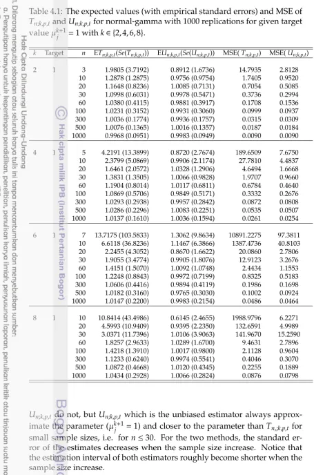
4.1 The expected values (with empirical standard errors) and MSE ofTn;k,p,tandUn;k,p,tfor normal-gamma with 1000 replications for given target valueµkj+1=1 withk∈ {2,4,6,8}. . . 44 4.2 The expected values (with empirical standard errors) and MSE
ofTn;k,p,tandUn;k,p,tfor normal-gamma with 1000 replications for given target valueµkj+1=5k+1withk∈ {2,4,6,8} . . . 46 4.3 The expected values (with standard errors) and MSE of Tn;k,p,t
and Un;k,p,t for normal inverse-Gaussian with 1000 replications for given target valueµk+2
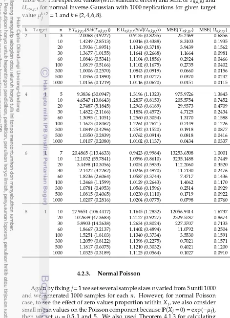
j =1 andk∈ {2,4,6,8}. . . 48 4.4 The expected values (with empirical standard errors) of Tn;k,p,t,
Un;k,p,t and Bn;k,p,t,α,β for normal-Poisson from 1000 replications for given target valueµkj=0.5k withk∈ {2,4,6,8},α=Xjandβ=k. 50 4.5 The empirical mean square errors (MSE) of Tn;k,p,t, Un;k,p,t and
Bn;k,p,t,α,βfor normal-Poisson from 1000 replications withµj=0.5, k∈ {2,4,6,8},α=Xjandβ=k. . . 51 4.6 The expected values (with empirical standard errors) of Tn;k,p,t,
Un;k,p,t and Bn;k,p,t,α,β for normal-Poisson from 1000 replications for given target valueµkj=1 withk∈ {2,4,6,8},α=Xjandβ=k. . 53 4.7 The empirical mean square errors (MSE) of Tn;k,p,t, Un;k,p,t and
Bn;k,p,t,α,β for normal-Poisson from 1000 replications with µj =1, k∈ {2,4,6,8},α=Xjandβ=k. . . 54 4.8 The expected values (with empirical standard errors) of Tn;k,p,t,
Un;k,p,t and Bn;k,p,t,α,β normal-Poisson from 1000 replications for
given target valueµkj =5kwithk∈ {2,4,6,8},α=Xjandβ=k. . . . 56 4.9 The empirical mean square errors (MSE) of Tn;k,p,t, Un;k,p,t and
Bn;k,p,t,α,β for normal-Poisson from 1000 replications with µj =5, k∈ {2,4,6,8},α=Xjandβ=k. . . 57
6.1 The expected values (and MSE) of bµj from 1000 replications for p=1,n∈ {30,50,100,300,500,1000,1500,2000}andk∈ {3,4,6,8} . . 74 6.2 The expected values (and MSE) of bµj from 1000 replications for
6.5 Fitting result for district households expenditure . . . 80 6.6 Comparison of bivariate dispersions between city and district . . 81 6.7 overall measure of dispersion estimates . . . 81
1.1 Research Roadmap . . . 4
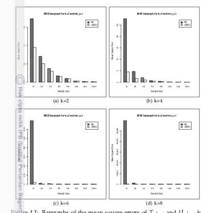
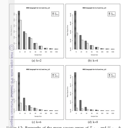
4.1 Bargraphs of the mean square errors of Tn;k,p,t and Un;k,p,t for normal-gamma withµj=1 andk∈ {2,4,6,8}. . . 45
4.2 Bargraphs of the mean square errors of Tn;k,p,t and Un;k,p,t for normal-gamma withµj=5 andk∈ {2,4,6,8}. . . 47
4.3 Bargraphs of the mean square errors of Tn;k,p,t and Un;k,p,t for normal inverse Gaussian withµj=1 andk∈ {2,4,6,8}. . . 49
4.4 Bargraphs of the mean square errors ofTn;k,p,t,Un;k,p,tandBn;k,p,t,α,β for normal-Poisson withµj=0.5 andk∈ {2,4,6,8}. . . 52
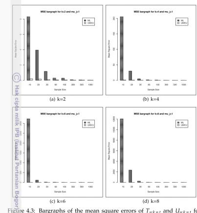
4.5 Bargraphs of the mean square errors ofTn;k,p,t,Un;k,p,tandBn;k,p,t,α,β for normal-Poisson withµj=1,k∈ {2,4,6,8}. . . 55
4.6 Bargraphs of the mean square errors ofTn;k,p,t,Un;k,p,tandBn;k,p,t,α,β for normal-Poisson withµj=5 andk∈ {2,4,6,8}. . . 58
6.1 Bargraph ofMSE(µbj) forp=1 andµj=0.5 . . . 76
6.2 Bargraph ofMSE(µbj) forp=1 andµj=1 . . . 76
6.3 Bargraph ofMSE(µbj) forp=1 andµj=5 . . . 76
6.4 Normality test of food expenditure for city households using histogram and Q-Q plot . . . 77
6.5 Normality test of nonfood expenditure for city households using histogram and Q-Q plot . . . 78
6.6 Cullen and Frey graph of food expenditure of city households . . 78
6.7 Cullen and Frey graph of nonfood expenditure of city households 79 6.8 Histogram, normal curve (- - -) and NIG curve (—-) . . . 80
6.9 Bivariate normal inverse-Gaussian distribution for expenditure of Bogor households data . . . 80
6.10 Histograms with normal and NIG curves . . . 82
LIST OF APPENDICES
A UNIVARIATE DISPERSION MODELS ... 89A.1 Univariate Exponential Dispersion Models ... 89
A.2 Univariate stable Tweedie models ... 91
B R CODES FOR SIMULATIONS ... 95
B.1 Generalized Variance Estimations ... 95
B.2 Estimation of Unobserved Univariate Stable Tweedie Mean... 104
C SCATTERPLOTS OF SOME GENERATED DATA... 110
1.1. Research Background
Multivariate data are commonly found in a variety of applied problems; they appear in the field of sociology, economy, agriculture, computer sci-ences and medical researches. In statistical analysis of multivariate data, along with measures of central tendency, measure of dispersion plays an important role in descriptive statistics and inferences. Dispersion denotes how stretched or squeezed is a distribution or data. The dispersion of multivariate data usually measured by covariance matrix and generalized variance (i.e. the determinant of the covariance matrix).
Many scientific publications devoted to the multivariate dispersion in-vestigations have been done for some decades, see e.g. Wilks (1932, 1967) for the introduction of generalized variance and a multivariate dispersion of multidimensional distributions, Mathai (1972); Behara and Giri (1983) for the statistical properties of Wilk’s generalized variance, Fernandez-Ponce and Suarez-Llorens (2003) for multivariate dispersion ordering based on quan-tiles and Gijbel and Omelka (2013) for the use of dissimilarity measures in testing for homogeneity of multivariate dispersions.
As one of the dispersion measures, generalized variance (i.e. the determi-nant of covariance matrix), is a scalar measure of dispersion for multivariate data (under normality) which was introduced by Wilks (1932); it is used for overall multivariate scatter and one can rank distinct groups and populations based on the order of their spread (Wilks, 1967). The uses of generalized vari-ance have been discussed by several authors. In sampling theory, Arvanitis and Afonja (1971) used generalized variance as a loss function in multipara-metric sampling allocation. In the theory of statistical hypothesis testing, Isaacson (1951) used generalized variance as a criterion for an unbiased crit-ical region to have the maximum Gaussian curvature. In the descriptive statistics, Goodman (1968) proposed a classification of some varieties of rice according to their generalized variances. Kokonendji and Seshadri (1996) and Kokonendji and Pommeret (2007) extended the generalized variance for non-normal distributions, in particular for natural exponential families (NEFs). Similar to variance functions of NEFs, characterizations and also estimations of generalized variance functions of NEFs become challenging problems.
Motivated by normal gamma and normal inverse Gaussian models, Boubacar Maïnassara and Kokonendji (2014) introduced a new form of gen-eralized variance functions which are generated by the so-called normal sta-ble Tweedie (NST) models ofk-variate distributions (k>1). As alternatives to multivariate normal model, the NST family is composed by distributions of random vectorX=(X1, . . . ,Xk)⊤ where Xj is a univariate (non-negative) stable Tweedie variable and (X1, . . . ,Xj−1,Xj+1, . . . ,Xk)⊤ =: Xcj given Xj are
k−1 real independent Gaussian variables with variance Xj, for any fixed
j∈ {1,2, . . . ,k}. Several particular cases have already appeared in different
contexts; one can refer to Boubacar Maïnassara and Kokonendji (2014) and references therein. However, some new statistical aspects of the family of NST models need to be investigated.
Among NST models, normal-gamma is the only model which is also a member of simple quadratic natural exponential families (NEFs) of Casalis (1996); she called it “gamma-Gaussian“ and it has been characterized by variance and generalized variance functions. See Casalis (1996) or Kotzet al. (2000, Chapter 54) for characterization by variance function, and Kokonendji and Masmoudi (2013) for characterization by generalized variance function which is the determinant of covariance matrix expressed in terms of the mean vector.
In contrast to normal-gamma which is the same to gamma-Gaussian; normal-Poisson and Poisson-Gaussian (Kokonendji and Masmoudi, 2006;
Koudou and Pommeret, 2002) are two completely different models. Indeed,
for any value of j∈ {1, . . . ,k}, a normal-Poisson model has only one
Pois-son component andk−1 Gaussian components, while a Poisson-Gaussianj
model has j Poisson components and k−j Gaussian components which
are all independent. Poisson-Gaussian is a particular case of the
sim-ple quadratic NEFs with variance functionVF(m)=diagk(m1, . . . ,mj,1, . . . ,1) wherem=(m1, . . . ,mk)⊤is the mean vector, and its generalized variance func-tion is detVF(m)=m1. . .mj. Some characterizations of Poisson-Gaussianj models have been done by several authors such as Letac (1989) for variance function, Kokonendji and Masmoudi (2006) for generalized variance func-tion, and Koudou and Pommeret (2002) for convolution-stability. Also one can see Kokonendji and Pommeret (2007); Kokonendji and Seshadri (1996) for the generalized variance estimators of Poisson-Gaussian. This normal-Poisson is also different from the purely discrete "Poisson-normal" model of
Steyn (1976), which can be defined as a multiple mixture ofkindependent
Poisson distributions with parametersm1,m2, . . . ,mk and those parameters have a multivariate normal distribution.
on the characterization of normal- Poisson models by variance function and generalized variance is presented in Chapter 5. Then we discuss two exam-ples of normal stable Tweedie models in Chapter 6.
1.2. Research Objectives
The objectives of this study were:
1. To investigate the multivariate exponential dispersion models, partic-ularly normal stable Tweedie models and their properties.
2. To determine the generalized variance estimators of some normal sta-ble Tweedie models and to analyze the effect of data dimensionkand
sample size n on the generalized variance estimation empirically by
simulation studies.
3. To investigate the characterization of normal Poisson models as a spe-cial case of NST models by variance function and by generalized vari-ance.
4. To apply the generalized variance estimation of NST models to real data.
1.3. Novelty
The novelties of this study were:
1. Empirical analysis of the generalized variance estimations of some normal stable Tweedie models using ML and UMVU estimators.
2. Bayesian generalized variance estimator of normal Poisson models.
3. Characterization of normal Poisson models by variance function and by generalized variance function.
1.4. Research Roadmap
In this chapter we emphasize some multivariate dispersion models pre-ceded by some basic relevant technical backgrounds.
2.1. Notion of Dispersion Measures
Dispersion concerns with how spread out or dispersed a distribution is. A statistic that conveys this information is a measure of dispersion. There are some measures of dispersion for univariate and multivariate data.
2.1.1. Univariate Dispersion
The simplest measure of univariate dispersion is therange, which is the difference between the greatest and the smallest values for a given variable, among thenobservations. It is a simple concept often used, but it does not tell us anything about the distribution of values of the variable of interest.
The commonly used measures of dispersion are the standard deviation and variance. The variance of a data set is calculated by taking the arithmetic
mean of the squared differences between each value and the mean value.
Because the differences are squared in variance calculation, the units of variance are not the same as the units of the data. Standard deviation is simply the square root of the variance and the units then correspond to those of the data set.
The calculation and notation of the variance and standard deviation depends on whether we are considering the entire population or a sample set. Following the general convention of using Greek characters to express population parameters and Arabic characters to express sample statistics, the notation for standard deviation and variance is as follows:
σ=population standard deviation
σ2=population variance
s=estimate of population standard deviation based on sampled data
s2=estimate of population variance based on sampled data
The population variance is defined as:
σ2= 1
N N X
i=1
xi−µ2
where µ = population mean, N= number of observations in population
(population size). The population standard deviation is the square root of this value.
The variance of a sampled subset of observations is calculated in a similar manner, using the appropriate notation for sample mean and number of observations. However, while the sample mean is an unbiased estimator
of the population mean, the same is not true for the sample variance if it is calculated in the same manner as the population variance. If one took
all possible samples of n members and calculated the sample variance of
each combination usingnin the denominator and averaged the results, the
value would not be equal to the true value of the population variance; that
is, it would be biased. This bias can be corrected by using (n−1) in the
denominator instead of justn, in which case the sample variance becomes
an unbiased estimator of the population variance. This corrected sample variance is defined as:
s2= 1 deviation is the square root of this value.
2.1.2. Multivariate Dispersion
A. Covariance Matrix and Dispersion Matrix
Let Xbe a random vector on Rk, i.e. X=(X1, . . . ,Xk), with mean vector
µ=E(X). Then the (theoretical) covariance matrix ofXis given by
Σµ=EX−µX−µ⊤
. (2.1)
This estimator of covariance matrix in (2.1) can be obtained from the observations in the sample using the following formula
Vn = 1 an unbiased estimator ofΣµ(Timm, 2002, p. 88).
Under normality, the maximum likelihood estimator of covariance matrix is given by
Although X is the unbiased and consistent ML estimator of µ, the ML
co-variance matrix estimator in (2.3) is a biased estimator ofΣµ.
Below we introduce a definition of dispersion matrix of a distribution
around a fixed point, then we also introduce the definition of its generaliza-tion.
moment exists. Then the dispersion matrix of Pθ around fixed point x0∈Rk is
equal to the covariance matrix in (2.1).
Definition 2.1.2. LetGbe a symmetric definite positive matrix. A generalization of dispersion matrix of Pθaround fixed pointx0∈Rkis given by:
We call (2.5) aG-dispersion matrix.
Properties
Notice that this estimator is the same as the sample covariance matrix
Vn of (2.2), i.e. Vn=bΣI,µ.
2. If G is unknown and we estimate it by ˆG, the G-dispersion matrix
estimator can be written as
bΣG,x
squared distances (Srivastava and Carter, 1983, p.232) between x0 and each observation.
Proposition 2.1.1. Let ΣG,x
0 be a G-dispersion matrix of κθ around fixed point
x0∈Rk. Then:
ΣG,x
0 =ΣG,µ+(µ−x0)G−
PROOF. We successfully have
B. Generalized Variance and Generalized Dispersion
Generalized variance is a scalar measure of dispersion for multivariate data (under normality) which was introduced by Wilks (1932); it is used for overall multivariate scatter and one can rank distinct groups and pop-ulations based on the order of their spread (Wilks, 1967). The generalized variance of ak-dimensional random vector variableXis defined as the deter-minant of its covariance matrix. It has an important role both in theoretical and applied research. In sampling theory, Arvanitis and Afonja (1971) used generalized variance as a loss function in multiparametric sampling allo-cation. In the theory of statistical hypothesis testing, Isaacson (1951) used generalized variance as a criterion for an unbiased critical region to have the maximum Gaussian curvature. In the descriptive statistics, Goodman (1968) proposed a classification of some varieties of rice according to their generalized variances. Kokonendji and Seshadri (1996) and Kokonendji and Pommeret (2007) extended the generalized variance for non-normal distri-butions in particular for natural exponential families (NEFs).
Definition 2.1.3. Thegeneralized varianceof Pθis given by:
detΣµ=det Z
Rk
x−µx−µ⊤Pθ(dx). (2.6)
The estimation of generalized variance is usually based on the determi-nant of the sample covariance matrixVn, i.e.
SinceE[detVn]<detΣµ (see e.g. Timm, 2002, p. 98), then detVn is a biased estimator.
Following the term of generalized variance for the covariance matrix, here we introduce definition of generalized dispersion for dispersion matrix.
Definition 2.1.4. The generalizedG-dispersionof Pθ around fixed pointx0 is given by
IfG=I, then the generalizedI-dispersion is simply the generalized dis-persion:
Moreover, ifG=Iandx0=µin Definition 2.1.4, then we have the generalized dispersion the same as the generalized variance in (2.6).
For the generalizedG-dispersion, the estimator is given by
[
Jørgensen (1986) introduced dispersion models as the class of error dis-tributions for the generalized linear models (GLM) which has drawn a lot of attention in the literature. The dispersion models contain many com-monly used distributions such as normal, Poisson, gamma, binomial, nega-tive binomial, inverse Gaussian, compound Poisson, von Mises and simplex distributions (Bandorff-Nielsen and Jørgensen, 1991).
The multivariate dispersion models generalize the univariate dispersion models (see Appendix A) which is based on the so-calleddeviance residuals:
r(x;µ)=[r(x1;µ1), . . . ,r(xk;µk)]⊤,
where xj and µj denote the elements of the k-vectors x and µ respectively andr(x;µ) is the univariate deviance residual.
Following Jørgensen and Lauritzen (2000) and Jørgensen (2013), we de-fine a multivariate dispersion model as follows:
Definition 2.2.1. Amultivariate dispersion modelDMk(µ,Σ)with position pa-rameterµand dispersion parameterΣis a family distribution forxwith probability density function of the form:
where a(x;Σ)is a suitable function such that (2.7) is a probability density function
The multivariate normal distribution is a special case of (2.8), i.e. by letting:
r(x;µ)=x−µ
a(Σ)=(2π)−k/2[det(Σ)]−1/2 b(x)=1
we obtaine the multivariate normal distribution:
f(x;µ,Σ)= 1
Jørgensen and Lauritzen (2000) introduced a simple notation for (2.7)
by using the scaled deviance as a quadratic form of the vector of deviance
residuals,
D(x;µ,Σ)=[r(x;µ)]⊤Σ−1r(x;µ)=trhΣ−1[r(x;µ)]⊤r(x;µ)i. (2.9) Using notation (2.9) then the multivariate dispersion models can be written as
They also showed that the matrix variance function corresponding to the scaled devianceDis
⊙ is the Hadamard (element-wise) product, and ˜V(µ) denotes the matrix
with elements [V(µi)]1/2[V(µj)]1/2fori;j=1, . . . ,k.
To generalize (2.7), Jørgensen and Lauritzen (2000) proposed a method for constructing multivariate proper dispersion models by using notation Λ=Σ−1instead of Σ. Then we writea(x;Λ) instead ofa(x;Σ) andD(x;µ,Λ) instead ofD(x;µ,Σ) and so on.
normalizing constanta(Σ) depends on the parameters only throughΣ. How-ever, this technique does not work for exponential dispersion models, calling for an alternative method of construction.
2.2.1. Multivariate Exponential Dispersion Models
Exponential dispersion models are particular cases of the dispersion models. Jørgensen in his book"The Theory of Dispersion Models"(1997) intro-duced two types of exponential dispersion models: additiveandreproductive exponential dispersion models. The multivariate form of these models was introduced by Jørgensen and Lauritzen (2000), and then discussed in details by Jørgensen (2013) and Jørgensen and Martínez (2013).
A. Ordinary Exponential Dispersion Models
Before we discuss these multivariate exponential dispersion models (EDM)
parameterized byµand Σ, we first need to understand the ordinary
expo-nential dispersion models which can be described as follow.
Consider a σ−finite measureνon R, the ordinary cumulant generating
function (CGF) for a randomk-vectorXis defined by
κ(θ)=κ(θ;X)=logEeθ⊤X for θ∈Rk,
with effective domainΘ={θ∈Rk:κ(θ)<∞}.
Theadditiveform of ak-variate exponential dispersion model is denoted byX∼ED∗(µ, λ) whereµis thek×1rate vector andλis the positiveweight pa-rameter(sometimes called the index or convolution parameter). This model is defined as a family distribution forXwith probability density/mass func-tion with respect to a suitable measure onRkas follows
f∗(x;θ, λ)=a∗(x;λ) exphx⊤θ−λκ(θ)i for x∈Rk, (2.10)
where a∗(x;λ) is a suitable function ofx and λ, and the cumulant function
κ(θ) depends on the canonical parameter θ∈Θ⊆Rk related to µ by the
following equation
µ=E(X)=κ′(θ) (2.11)
andλhas domainR+
We note that the model ED∗(µ, λ) hask+1 parameters, of which the single parameterλcontrols the covariance structure of the distribution. The mean vector of (2.10) isλµand the covariance matrix isλV(µ) with
V(µ)=κ′′◦κ′(µ) (2.12)
The CGF of ED*(µ, λ) satisfies
λκ(s;θ)=λ[κ(s+θ)−κ(θ)] for s∈Θ−θ (2.13)
which is finite for the argumentsbelonging to a suitable neighborhood of
zero, and hence characterizes the distribution in question. It also follows from (2.13) that the model ED∗(µ, λ) satisfies the following additive property:
ED∗(µ, λ1)+ED∗(µ, λ2)=ED∗(µ, λ1+λ2) for λ1, λ2>0
For each additive exponential dispersion model ED∗(µ, λ), the corre-spondingreproductive exponential dispersion modelED(µ, σ2) is defined by the duality transformationY=λ−1X, or
ED(µ, σ2)=λ−1ED∗(µ, λ)
whereσ2=1/λis called thedispersion parameter.
Thereproductiveform of ak-variate exponential dispersion model denoted by ED(µ, σ2) withlocationparameterµanddispersionparameterσ2is defined as a family distribution forYwith probability density/mass function onRk
of the form
f(y;θ, λ)=a(y;λ) expnλhy⊤θ−κ(θ)io for y∈Rk, (2.14)
with respect to a suitable measure onRk, wherea(y;λ) is a suitable function
ofyandλ. The random vectorYon (2.14) has meanµand variance
Var(Y)=σ2V(µ).
The model ED(µ, σ2) satisfies the following reproductive property (see Jørgensen and Martínez, 2013):
I f Y1, . . . ,Yn are i.i.d.ED(µ, σ2), then 1
n n X
i=1
Yi∼ED(µ, σ2/n).
To provide a fully flexible covariance structure corresponding to a mean vectorµand a positive-definite dispersion matrixΣ, an alternative method for the construction of multivariate exponential dispersion model is needed. Jørgensen and Martínez (2013) discussed a detail construction for multivari-ate exponential dispersion models which are very helpful and important for understanding this family of distribution. With this method then the covari-ance matrix of EDM is of the form Cov(X)=Σ⊙V(µ), where⊙denotes the
Hadamard (element-wise) product between two matrices, andV(µ) denotes
B. Multivariate Additive Exponential Dispersion Models
The construction of multivariate additive exponential dispersion model is based on an extended convolution method, which interpolates between the set of fully correlated pairs of variables and the set of independent mar-gins of the prescribed form so that the marginal distributions follow a given univariate exponential dispersion model. This method explores the con-volution property of conventional additive exponential dispersion models
in order to generate the desired number of parameters, namely k means
and k(k+1)/2 variance and covariance parameters. Multivariate additive
exponential dispersion models are particularly suitable for discrete data, and include multivariate versions of the Poisson, binomial and negative binomial distributions.
We start by the extended convolution method in the bivariate additive case as described by Jørgensen and Martínez (2013) and Jørgensen (2013). Suppose that we are given an ordinary bivariate additive ED∗(µ, λ) with CGF
(s1,s2)⊤7→λκ(s1,s2;θ1, θ2)=λ[κ(s1+θ1,s2+θ2)−κ(θ1, θ2)].
From this model we define a multivariate additive exponential dispersion (bivariate case) by means of the following stochastic representation for the random vectorX:
where the three vectors on the right-hand side of (2.15) are assumed inde-pendent. More precisely, withθ=(θ1, θ2)⊤and theweight matrix:
The equation (2.16) above is interpreted as interpolating between inde-pendence (λ12=0) and the maximally correlated case (λ1=λ2=0). We note that the margins have the same form as forλκ(s1,s2;θ1, θ2), as seen from the two marginal CGFs as follow
K(s1,0;θ,Λ)=(λ12+λ1)κ(s1,0;θ1, θ2)=λ11(s1,0;θ1, θ2) K(0,s2;θ,Λ)=(λ12+λ2)κ(0,s2;θ1, θ2)=λ22(0,s2;θ1, θ2)
while replacing the single parameterλ by the three parameters ofΛ, for a total of five parameters.
Using the notation (2.11), the mean vector forXis
E(X)=diag(Λ)µ= additive exponential dispersion defined by (2.16), parametrized by the rate vectorµand weight matrixΣ.
The covariance matrix forXis
Var(X)=
where theVij are elements of the unit variance function defined by (2.12). The correlation betweenX1andX2is
Corr(X1,X2)= √λ12 may be either positive or negative, depending on the sign ofV12(µ).
Now let us consider for the trivariate case, following Jørgensen (2013) we define the trivariate random vector X=(X1,X2,X3)⊤ as the sum of six
of which three terms are bivariate and three are univariate. However, rather than starting from a trivariate CGFκ(s1,s2,s3;θ) as was done by (Jørgensen, 2013), Jørgensen and Martínez (2013) started from the three bivariate distri-butions corresponding to the first three terms (2.17). For this construction to work, it is crucial that the univariate margins of the three bivariate terms are consistent, so that for exampleU11 and U21 have distributions that belong to the same class. In order to avoid the intricacies of such a construction in the general case, we concentrate here on the homogeneous case, where all three margins belong to the same class, for example a multivariate gamma distribution with gamma margins.
ED∗3(µ,Λ) is defined via the joint CGF for the vectorXas follows:
K(s1,s2,s3;µ,Λ)=λ12κ(s1,s2;µ1, µ2)+λ13κ(s1,s3;µ1, µ3)+λ23κ(s2,s3;µ2, µ3)+
λ1κ(s1, µ1)+λ2κ(s2, µ2)+λ3κ(s3, µ3)
This definition satisfies the requirement that each marginal distribution belongs to the univariate model ED∗(µ, λ). For example, the CGF of the first margin is
K(s1,0,0;µ,Λ)=λ12κ(s1,0;µ1, µ2)+λ13κ(s1,0;µ1, µ3)+λ23κ(0,0;µ2, µ3)+
λ1κ(s1, µ1)+λ2κ(0, µ2)+λ3κ(0, µ3)
=λ12κ(s1, µ1)+λ13κ(s1, µ1)+λ1κ(s1, µ1)
While all three bivariate marginal distributions are of the form (2.16). For example, the CGF of the joint distribution ofX1andX2is
K(s1,s2,0;µ,Λ)=λ12κ(s1,s2;µ1, µ2)+λ13κ(s1,0;µ1, µ3)+λ23κ(s2,0;µ2, µ3)+
λ1κ(s1, µ1)+λ2κ(s2, µ2)+λ3κ(0, µ3)
=λ12κ(s1,s2;µ1, µ2)+(λ1+λ13)κ(s1, µ1)+(λ2+λ23)κ(s2, µ2),
which has rate vector (µ1, µ2)⊤ and weight matrix given by the upper left 2×2 block ofΛ.
Based on these considerations (the construction for bivariate and trivari-ate cases), the multivaritrivari-ate exponential dispersion model ED∗k(µ,Λ) for gen-eralkis defined as the following.
Definition 2.2.2. An additive k-variate exponential dispersion model ED∗k(µ,Λ) with k×1rate vectorµ=(µ1, . . . , µk)⊤ and k×k weignt matrixΛ={λij}ki,j=1, is a family distribution with a joint cumulant generating function of the form
K(s;µ,Λ)=X i<j
λijκ(si,sj;µi, µj)+
k X
i=1
λiκ(si, µi), (2.18)
where all weightsλijandλiare positive, withλii=Pj;j,iλij+λi,
The mean vector of (2.18) is
E(X)=diag(Λ)µ,
where diag{Λ} is a k×k diagonal matrix. By arguments similar to those
given in the trivariate case above it can be shown that each univariate margin belongs to the univariate model ED∗(µ, λ), and that all marginal distributions for a subset of thekvariables are again of the form (2.18).
prop-erty
ED∗k(µ,Λ1)+ED∗k(µ,Λ2)=ED∗k(µ,Λ1+Λ2). (2.19) From (2.18) we find that fori, jtheijth covariance is
Cov(X1,Xj)=λijV(µi, µj),
whereV(µi, µj)=κ′′(0,0;µi, µj) denotes the second mixed derivative ofκ(·,·;µ1, µ2)
at zero. Generalizing (2.2), the covariance matrix for X may hence be
ex-pressed as a Hadamard product,
Var(X)=Λ⊙V(µ),
where the (matrix) unit variance functionVnow has diagonal elementsV(µi) and off-diagonal elementsV(µi, µj).
This construction done by Jørgensen (2013) gives us exactly the desired number of parameters, namelykrates andk(k+1)/2 covariance parameters.
C. Multivariate Reproductive Exponential Dispersion Models
The reproductive form of multivariate exponential dispersion model is constructed by applying the so-calledduality transformationto a given mul-tivariate additive exponential dispersion model. The reproductive form is particularly suited for continuous data, and includes the multivariate nor-mal distribution as a special case, along with new multivariate forms of gamma, inverse Gaussian and other Tweedie distributions.
A multivariate exponential dispersion model in its reproductive form is
parameterized by ak-vector of meansµ and a symmetric positive-definite
k×k dispersion matrix Σ. We shall now derive the reproductive form of
whereΣis the symmetric positive-definite matrix defined by
and 3 variance-covariance parameters. We hence call this five-parameter family abivariate reproductive exponential dispersion model.
To obtain a general multivariate reproductive form of exponential dis-persion models, we use a generalization of the ordinary duality transfor-mation (2.2). By using a k×k diagonal matrix diag(Λ) from above, define the reproductive multivariate exponential dispersion model EDk(µ,Σ) by the (extended) duality transformation
EDk(µ,Σ)=Diag(Λ)−1ED∗
k(µ,Λ) (2.20)
The reproductive model EDk(µ,Σ) has mean vector µ and dispersion
matrix Σ =diag(Λ)−1Λdiag(Λ)−1. It satisfies the following reproductive
According to the duality transformation (2.20), each additive exponential dispersion model ED∗k(µ,Λ) has a corresponding reproductive counterpart. The inverse duality transformation is given by
ED∗k(µ,Λ)=Diag(Λ) EDk(µ,Diag(Λ)−1ΛDiag(Λ)−1)
by which the additive form ED∗k(µ,Λ) may be recovered from the reproduc-tive form.
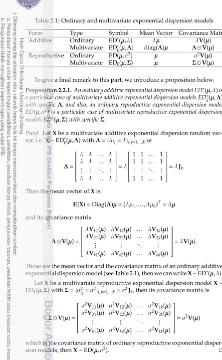
Table 2.1: Ordinary and multivariate exponential dispersion models
Form Type Symbol Mean Vector Covariance Matrix
Additive Ordinary ED∗(µ, λ) λµ λV(µ)
Multivariate ED∗k(µ,Λ) diag(Λ)µ Λ⊙V(µ)
Reproductive Ordinary ED(µ, σ2) µ σ2V(µ)
Multivariate EDk(µ,Σ) µ Σ⊙V(µ)
To give a final remark to this part, we introduce a proposition below.
Proposition 2.2.1. An ordinary additive exponential dispersion model ED∗(µ, λ)is a particular case of multivariate additive exponential dispersion models ED∗k(µ,Λ) with specific Λ, and also, an ordinary reproductive exponential dispersion model ED(µ, σ2) is a particular case of multivariate reproductive exponential dispersion models EDk(µ,Σ)with specificΣ.
Proof. Let Xbe a multivariate additive exponential dispersion random vec-tor, i.e. X∼ED∗k(µ,Λ) withΛ={λij=λ}i,j=1,...,kor
Then the mean vector ofXis:
E(X)=Diag(Λ)µ= λµ1, . . . , λµk⊤=λµ
Those are the mean vector and the covariance matrix of an ordinary additive exponential dispersion model (see Table 2.1), then we can writeX∼ED∗(µ, λ).
Let Xbe a multivariate reproductive exponential dispersion modelX∼
EDk(µ,Σ) withΣ={σ2ij=σ2}i,j=1,...,k=σ2Jk, then its covariance matrix is
which is the covariance matrix of ordinary reproductive exponential
D. Multivariate Tweedie Models: an Example
In this part we discuss the multivariate Tweedie models as special cases of multivariate EDM. First we recall that the univariate Tweedie models are particular cases of univariate EDM which admit the power unit variance function:
V(µ)=µp (2.21)
withp∈(−∞,0]∪[1,∞) is called thepower parameter. The domain forµisR
forp=0 andR+for other values ofp. The cumulant function and mean can
be found for univariate Tweedie models by equatingκ′′(θ)=dµ/dθ=µpand solving forµandκ. We define clearly the univariate stable Tweedie models below.
Definition 2.2.3. Let t>0 be the convolution parameter and the index parameter
α∈[−∞,1)∪(1,2] intrinsically connected to the power variance parameter p∈ for allθ0in their respective canonical domains
Θ(νp,1)=
Some details and examples of univariate Tweedie models are given in Ap-pendix A.
bivariate singular distribution with joint CGF
whose marginals are Tweedie distributions of the form (2.24). Now we define the multivariate Tweedie models as follow.
Definition 2.2.4. Amultivariate (additive) Tweedie modeldenoted Tw∗kp(µ,Λ) is defined by the joint CGF:
K(s;θ, γ)=X marginal follows a univariate Tweedie distribution with CGF (2.24) with
θ=θiandγ=γii defined by
γii=
X
j:j,i
γij+γi.
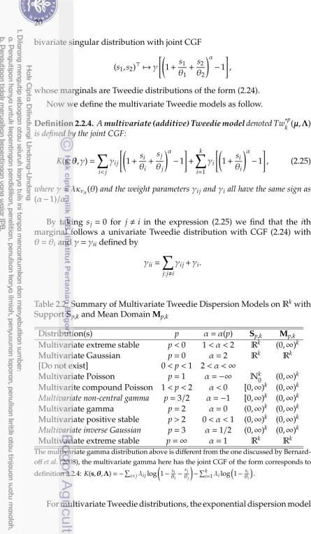
Table 2.2: Summary of Multivariate Tweedie Dispersion Models onRkwith
SupportSp,kand Mean DomainMp,k
The multivariate gamma distribution above is different from the one discussed by Bernard-offet al.(2008), the multivariate gamma here has the joint CGF of the form corresponds to definition 2.2.4:K(s,θ,Λ)=−Pi<jλijlog
weight parametersλiiandλijare defined by
Using the parametersλii the marginal mean are of the form
λiiµi=λiiκα(θi)θα with mean vector Diag(Λ)µwhere its elements are defined by (2.28), i.e.
Diag(Λ)µ= λ11
and the covariance matrix for Xhas the formΛ⊙V(µ), where the elements ofΛ=(λij)i,j=1,...,kare defined in (2.26) and (2.27) andV(µ) has entries
Vij=(µiµj)p/2, then the covariance matrix ofXis
Σ=Λ⊙V(µ)=
The multivariate additive Tweedie modelTw∗kp(µ,Λ) satisfies the follow-ing additive property:
To obtain the reproductive formTwk(µ,Σ), we need to use the following
One can see Jørgensen and Martínez (2013) and Cueninet al. (2016) for
more details on multivariate Tweedie models. An interesting behavior of negatively correlated multivariate Tweedie distribution (bivariate case) was
revealed from the simulation study done by Cuenin et al. (2016). They
showed that for a large negative correlation the scatter of bivariate Tweedie distribution depicted a curve which reminds us to the inverse exponential function, also the distribution lies only on the positive side of the Euclidean space. These behaviour appears to be new because of positive support of the multivariate Tweedie. While for large positive correlation the scatter of bivariate Tweedie distribution depicted a straight line with positive slope as commonly seen in the same case on multivariate Gaussian distribution.
2.2.2. Multivariate Geometric Dispersion Models
The dispersion models for geometric sums are defined as two-parameter families that combine geometric compounding with an operation called geometric tilting, in much the same way that exponential dispersion models combine convolution and exponential tilting (Jørgensen, 1997, Chap.3). The univariate geometric dispersion model was introduced by Jørgensen and Kokonendji (2011).
A. Definition and Properties
A multivariate geometric sums(Q) (Kalashnikov, 1997, page 3), indexed by the probability matrixQ, can be defined by
N(Q) has probability mass function to be defined. Note that each of the sums (2.29) must be ordinary geometric sums with probability parameters
q11, . . . ,qkk.
The geometric random vectorN(Q) has probability mass function:
P[n1(Q), . . . ,nk(Q)]=
[Pki=1ni(Q)]! Qk
i=1ni(Q)! k Y
i=1 qni(Q)
i (1−q1−. . .−qk)
where ni(Q)∈N={0,1,2, . . .}(the set of natural numbers),qi>0,i=1, . . . ,k,
andPki=1q1<1 (Sreehari and Vasudeva, 2012).
For this section, we denote again the ordinary CGF for a randomk-vector
Xby
κ(s)=κ(s;X)=logEes⊤X for s∈Rk, (2.30)
with effective domainΨ ={s∈Rk:κ(s)<∞}.
Definition 2.2.5. IfXis a k-variate random vector, the geometric cumulant function (GCF) forXis given by
G(s)=G(s;X)=1−e−κ(s) for s∈ D(G),
with domainD(G)={s∈Rk:G(s)<1}= Ψ.
Recall that a CGF is a real analytic convex function, which is strictly convex unless X is degenerate (concentrated on an affine subspace of Rk).
Hence, G is also real analytic, and the domainD(G), like Ψ, is convex. In fact, the gradient G′(s)=e−κ(s)κ′(s) is proportional to κ′((s)) in the interior int[D(G)]. Hence, by the convexity of κ, the GCF G is either sloping or cup-shaped.
When0∈int[D(G)], the derivativesG(n)(0)=G(n)(0;X) are called the geo-cumulantsofX.In particular, the first geo-cumulant is the mean vector,
G′(0)=κ′(0)=E(X).
The second geo-cumulant (called the geo-covariance) is thek×kmatrix
S(X)=G′′(0)=κ′′(0)−κ′(0)κ′⊤(0)=Var(X)−E(X)E⊤(X)
which satisfies the inequalities
−E(X)E⊤(X)6S(X)6Var(X).
The geo-covarianceS(X) satisfies a scaling relation similar to the covariance,
namely for anyℓ×kmatrixAwe have
As noted by Klebanovet al. (1985), the exponential distribution plays the role of degenerate distribution for multivariate geometric sums. Here we let Exp(µ) denote the distribution with GCF
G(s)=s⊤µ for s⊤µ<1
which forµ,0corresponds to a unit exponential variable multiplied onto
the vector µ, while µ=0 corresponds to the degenerate distribution at 0.
We refer to GCFs of the form (2.2) as thedegenerate case. Since S(X)=0for
X∼Exp(µ), we may interpret the operator S(X)=Var(X)−E(X)E⊤(X) as a
general measure of the deviation of the random vectorXor its distribution from exponentiality.
The multivariate Tweedie characteristic as special cases of exponential dispersion models can also be applied to the family of geometric dispersion
models, which can be so-called multivariate geometric Tweedie models. The
theoretical aspects of this new class of distribution need to be explored and would become an interesting work.
2.2.3. Multivariate Discrete Dispersion Models
Discrete dispersion models are two-parameter families obtained by com-bining convolution with a factorial tilting operation. Using the factorial cumulant generating function, Jørgensen and Kokonendji (2016) introduced a dilation operator, generalizing binomial thinning, which may be viewed as a discrete analogue of scaling. The discrete Tweedie factorial dispersion models are closed under dilation, which in turn leads to a discrete Tweedie asymptotic framework where discrete Tweedie models appear as dilation limits.
A. Definition and Properties
Before looking to the definition, let us recall that the CGF (2.30) satisfies the linear transformation law
κ(t,AX+b)=κ(At;X)+bt
whereAis a diagonal matrix.
Definition 2.2.6. If X is a k-variate random vector, and s a k-vector with non-negative elements, we use the notationfX= fX1
1 . . .f
Xk
k . The multivariate factorial cumulant generating function (FCGF) is defined by
C(t)=C(t;X)=logEh(1+t)Xi=κ log(1+t);X for t>−1
We should note that C, likeκ, characterizes convolution additively, i.e.
for independent random variablesXandYwe have
C(t;X+Y)=C(t,X)+C(t,Y).
The CGFκis a real analytic convex function and strictly convex unlessXis degenerate. Hence Cis also real analytic, and the domain D(C), like Ψ, is an interval. The derivative C′(t)=κ′(log(1+t))/(1+t) has the same sign as
κ′(log(1+t)) onint(D(C)). Hence, by the convexity ofκ, the FCGFCis either monotone or u-shaped.
When 0∈ int[D(C)], the derivatives C(n)(0) = C(n)(0;X) are called the factorial-cumulantsofX.The first factorial-cumulant is the mean vector,
C′(0)=κ′(0)=E(X),
and the second factorial-cumulant is thek×k dispersionmatrix
S(X)=C′′(0)=Cov(X)−diagE(X)
with entries
Sij(X)= (
S(Xi) for i= j Cov(Xi,Xj) for i, j.
Jørgensen and Kokonendji (2011) introduced a new definition of multi-variate over/under dispersion based on the dispersion matrix, namely that the random vectorXisequidispersedifS(X)=0,Xis calledover/underdispersed if the dispersion matrixS(X) is positive/negative semidefinite, i.e. S(X) has at least one positive/negative eigenvalue, respectively. Also, we say that the dispersion ofXisindefiniteifS(X) has both positive and negative eigenvalues. The dispersion matrix S(X) satisfies a scaling properties with respect to dilation. For a random vectorX, thedilation linear combinationc Xwith 1×k vectorcis defined as follows:
C(t;c·X)=C(c⊤t;X)
provided that the right-hand side is a (univariate) FCGF. The mean and dispersion matrix of a dilation linear combination are given by
E(c·X)=cE(X) and S(c·X)=c S(X)c⊤
respectively. It follows that if c·X is equidispersed for some c,0, then the dispersion matrixS(X) is singular. The reverse implication holds if the vector c>0is such that cS(X)c⊤=0.Similarly, for an ℓ×kmatrixA≥0we defineA·Xby
C(t;A X)=C(A⊤t;X),
B. Multivariate Poisson Tweedie models
Multivariate Poisson Tweedie models (Jørgensen and Kokonendji, 2011) are special cases of multivariate discrete dispersion models. The models are considered as a new class of multivariate Poisson-Tweedie mixtures, which is based on the multivariate Tweedie distributions of Jørgensen and Martínez (2013). Consider thek-variate Tweedie distributionY∼Twp(µ,Σ)
with mean vectorµand covariance matrix
Cov(Y)=Diag(µ)p/2ΣDiag(µ)p/2. (2.31)
Table 2.3: Summary of Multivariate Poisson Tweedie Models
Model p Type
Multivariate Neyman Type A p=1 +
Multivariate Poisson-Compound Poisson 1<p<3/2 +
Multivariate Pólya-Aeppli p=3/2 +
Multivariate Poisson-compound Poisson 3/2<p<2 +
Multivariate negative binomial p=2 +
Multivariate factorial discrete stable p>2 +
Multivariate Poisson-inverse Gaussian p=3 +
The multivariate Poisson-Tweedie modelPTp(µ,Σ) is defined as a Poisson mixture
X|Y∼ independent Po(Yi) for i=1, . . . ,k,
whereX1, . . . ,Xkare assumed conditionally independent givenY. The mul-tivariate Poisson-Tweedie model has univariate Poisson-Tweedie margins, Xi∼PTp(µi, σii) where σij denote the entries ofΣ.The mean vector is µand the dispersion matrix is (2.31) (positive-definite) making the distribution
overdispersed. The covariance matrix forXhas the form
Cov(X)=Diag(µ)+Diag(µ)ΣDiag(µ),
making it straightforward to fit multivariate Poisson-Tweedie regression models using quasi-likelihood. The multivariate Poisson-Tweedie model satisfies the following dilation property:
Diag(c)PTp(µ,Σ)=PTphDiag(c)µ,Diag(c)1−p/2ΣDiag(c)1−p/2i, wherecis ak-vector with positive elements.
2.2.4. Applications
Stochastic model for heterogeneities in regional organ blood flow
The theory of exponential dispersion models was applied to construct a stochastic model for heterogeneities in regional organ blood flow (Kendal, 2001). Regional organ blood flow exhibits a significant degree of spatial heterogeneity when measured by using labeled microspheres or by other means. The related velocity distribution of blood flow has been character-ized by a gamma distribution. To provide a stochastic description for the macroscopic and microscopic heterogeneities in regional organ blood flow, a scale invariant compound Poisson-gamma distribution was employed.
Distribution of human single nucleotide polymorphisms
A scale invariant Poisson gamma (PG) exponential dispersion model was used in modeling the distribution of human single nucleotide poly-morphisms (NSPs) (Kendal, 2003). The SNPs appear to be non-uniformly dispersed throughout the human genome, this non-uniformity can be at-tributed to a segmented genealogical substructure within the genome, where older segments may have accumulated greater numbers of SNPs. An analy-sis of 1.42 million human single nucleotide polymorphisms (SNPs) revealed an apparent power function relationship between the estimated variance and mean number of SNPs per sample bin. By PG-EDM model the sample bins contain random (Poisson distributed) numbers of identical by descent genomic segments, each with independently gamma distributed numbers of SNPs.
Geometricα-Laplace marginals in autoregressive process
Geometric Laplace distribution is one of the geometric dispersion model. Lekshmi and Jose (2004) proposed the used of geometric Laplace distribution as stationary marginal in autoregressive process modeling. Some contexts of applications were mentioned in their paper, e.g. for modeling pooled position errors in a large navigation system, for modeling sulphate concen-tration data with ARMA model, and for modeling financial time series data (see Hsu (1979), Damsleth and El-Shaarawi (1989), Anderson and Arnold (1993) respectively for details).
Integer valued time series modeling
In this chapter, we present the family of normal stable Tweedie models which is the extension of normal gamma (Bernardo and Smith, 1993) and
normal inverse Gaussian (Bandorff-Nielsen et al., 1982) models. Normal
Stable Tweedie (NST) models are composed by a fixed univariate stable Tweedie variable having a positive value domain, and the remaining random variables given the fixed one are real independent Gaussian variables with the same variance equal to the fixed component.
A random variableXis said to be stable (or to have a stable distribution) if it has the property that a linear combination of two independent copies of the variable, e.g. aX1+bX2 whereX1 andX2are two independent copies of X, has the same distribution with cX+d for some positive c and d∈R
(Nolan, 2017). The stable distribution family is also sometimes referred to as the Lévy alpha-stable distribution. While Tweedie distributed variable is a variable that belongs to the exponential dispersion family of distribution with specific power mean-variance relationships, i.e,V(µ)=µp(see Chapter 2, Equation 2.21) for somep. Then Tweedie distribution is to the subclass of the exponential dispersion models that admits a power variance function
V(µ)=µp (Jørgensen, 1997). Some details on univariate stable Tweedie
models are given in Appendix A.
3.1. Definition and Properties
Motivated by normal gamma and normal inverse Gaussian models, Boubacar Maïnassara and Kokonendji (2014) introduced a new form of
gen-eralized variance functions which are generated by the so-called normal
stable Tweedie(NST) models ofk-variate distributions (k>1). The generating
σ-finite positive measureµα,t onRkof NST models is composed by the well-known probability measureξα,t of univariate positiveσ-stable distribution generating Lévy process Xαt
t>0 which was introduced by Feller (1971) as follows
ξα,t(dx)= 1
πx
∞
X
r=0
trΓ(1+αr)sin(−rπα)
r!αr(α−1)−r[(1−α)x]αr1x>0dx=ξα,t(x)dx, (3.1)
whereα∈(0,1) is the index parameter,Γ(.) is the classical gamma function,
and IA denotes the indicator function of any given event A that takes the
value 1 if the event occurs and 0 otherwise. Parameterαcan be extended into
α∈(−∞,2] (see Tweedie, 1984). Forα=2, we obtain the normal distribution with density
ξ2,t(dx)= √1
2πtexp
−x2 2t
! dx.
For ak-dimensional NST random vectorX=(X1, . . . ,Xk)⊤, the generating