Research Title
:
Examination of Land Degradation based on
Erosion Potential using Revised Universal Soil
Loss Equation
(A Study Case of Bandung Regency, West Java,
Indonesia)
Name
:
Yee Yee Maw
Student ID
:
G 051048021
Study Program
:
Master of Science in Information Technology for
Natural Resources Management
Approved by,
Advisory Board
Dr. Ir. Tania June ,M.Sc
Iwan Setiawan ,S.Si,PM
Supervisor
Co-supervisor
Endorsed by,
Program Coordinator
Dean of the Graduate School
STATEMENT
I, Yee Yee Maw, here by stated that this thesis entitled:
Examination of Land Degradation Based on Erosion Potential Using Revised
Universal Soil Loss Equation (Case study Bandung Regency, West Java, Indonesia)
Are result of my own work during the period of January to May 2006 and that it has not
been published before. The content of the thesis has been examined by the advising
committee and the external examiner.
Bogor, June 2006
ACKNOWLEDGEMENT
First, I would like to express my deepest gratitude to Buddha the All Mighty for
His Mercy, Favor, Blazing me to carry out this task with sound health.
I wish to express my Earnest thanks and Sincere appreciation to the Government
of the Union of Myanmar,
Minister
and
Deputy Minister for Ministry of Agriculture
and Irrigation, my special Kind and Respected to
Mr. Tin Htut Oo, the
Director
General for Dept. of Agricultural Planning, Myanmar for their official endorsement,
kindly permission, allowed me to attend the Master for Information Technology for
Natural Resources Management Study Program in Bogor Agricultural University (IPB),
Indonesia.
I am very grateful to those who have helped me throughout this research period.
My especially gratitude and appreciation due to
Dr. Ir. Tania June
(Program
Coordinator of MIT) and
Ir. Iwan Setiawan
who acted respectively as my respected
Chairman and Member of Advisory committee. I am deeply appreciate and respected
them for their constant guidance, continuous encouragement, interest, and support during
the work and for providing the study area data throughout the duration of this project. I
really wish there were some way of showing my gratitude for all they have done for me.
I am especially grateful to my sponsor "
ASEAN FOUNDATION
" for financial
support by awarding me the Scholarship during of my two years Master Degree study
which without this support, this Degree would not be possible. I am deeply appreciated.
My special thanks goes to the
Director
,
Deputy Directors
, and
staffs
at the
SEAMEO Regional Center for Tropical Biology (SEAMEO BIOTROP). Also the MIT
staffs for their help and support to me during my study period in Indonesia. I thank very
much to
Drs Eddy Nugroho
and Dr. Budi Kartiwa
(Hydrology Research Lab) who
took their personal time to track down knowledge and provide insight and support
Citarum watershed metrology data. Without their assistance during some trying times, the
results of my work would have been less than desirable.
My special dedication and gratit ude goes to my sister,
Ms. Tin Tin Win
, the
cheerful lady who stream spirit, and provided as accompanied me during my
hard-pressed time. My profound gratitude goes to my friends in MIT 2004 odd and even
semester; 2005 even semester students, especially Mr. Adang Setiawan, Wen Wen and
Tran Xung Sang. I really grateful to appreciate for the advice, assistance and camaraderie
and best wishes to you all.
Curriculum Vitae
Yee Yee Maw was born in Yangon, Myanmar at June 6, 1974 as a
second daughter of U Kyaw Hla and Daw Khin Khin Myint. She
receives her undergraduate Degree from Yezin Agricultural
University in 1998 in the field of Soil and Water Management.
From the year of 1998 to present, she works for Department of
Agricultural Planning under the Ministry of Agricultural and Irrigation as a deputy
program office in Trade and Marketing Section.
ABSTRACT
YEE YEE MAW(2006).
Examination of Land Degradation Based on Erosion
Potential Using Revised Universal Soil Loss Equation (Case study Bandung
Regency, West Java, Indonesia).
Under the supervision of Dr. Ir. TANIA JUNE and
IWAN SETIAWAN.
Soil erosion is a serious environmental problem in the world. With the generally
high erosion rate in many parts of the world, efforts should be directed towards curtailing
its hazard. This requires quantitative data to identify critical areas where urgent
conservation is needed. Traditional approaches based on runoff plots are expensive, time
consuming and generate point-based data. A comparative study was conducted to
estimate soil loss under landscapes, major land uses and slope gradients in Bandung
Regency, West Java Province, Indonesia. The soil erosion model,
i.e
. the Revised
Universal Soil Loss Equation (RUSLE) was applied in GIS and remote sensing (RS)
environment.
GIS based spatial analysis model is used to answer questions about what exists
now or exists at some points in the past. Perhaps most importantly, it can be used to
predict what will happen or has happened in another location or at another point in a
certain time. A GIS provides these capabilities by means of its spatial analysis function.
Erosion that is caused by rain and human’s activities can be assessed with the Revised
Universal Soil Loss Equation in ton/hectare/year units based on soil loss rate of a certain
area. RUSLE involves erosivity from rain, erodibility from soil properties, slope
conditions, land conservation, and cultivation system factors on a land.
The classification of land cover in study area was conductive by using Landsat
satellite image of different years, i.e.1989, 1993, 1998 and 2003. Changes in land use/
cover was led to increase the rate of erosion by water in the Bandung regency which
could be concluded from the statistical analysis of the annual result from RUSLE. The
potential eroded area by districts in the study area can be examined. Human factor, land
use and cover change, is the most dominant factor in RUSLE equation for prediction of
land degradation was shown in the sensitivity analysis of land use/cover change by years.
TABLE OF CONTENTS
STATEMENT... I
ACKNOWLEDGEMENT ... II
CURRICULUM VITAE...III
ABSTRACT...IV
TABLE OF CONTENTS... V
LIST OF TABLE...VI
LIST OF FIGURE...VII
REFERENCES
……….88 – 94
LISTOFFIGURE
FIG(1.1):THE EROSION ASSESSMENT RATE OCCURRENCE IN WEST JAVA AREA
(JAWA BARAT)...6
FIG (2.1):DISTRIBUTION OF RAIN EROSION THROUGHOUT THE WORLD (HUDSON 1995)...10
FIG (3.1):THE GENERAL INFORMATION OF RUNOFF EROSION MODEL BASED ON SPATIAL ANALYSIS...16
FIG (3.1):THE LOCATION OF STUDY AREA...28
FIG (3.2):THE FLOW CHART OF THE WHOLE PROCEDURE OF STUDY...31
FIG (3.3):THE PROCESS OF DRIVIN G DIGITAL TERRAIN MODEL (DEM) FROM CONTOUR LINE MAP...32
FIG (3.4):THE FLOW CHART OF PREDICTION EROSION PROCESS BY RUSLE MODEL...36
FIG (3.5):THE PROCESS OF MANIPULATE LS FACTOR FROM DEM ...40
Fig (4.1): Flow Chart of Image Preprocessing ...44
Fig (4.2): The geometric correction image of 1989 and 1993 ...45
Fig (4.3): Images after geometric rectification of the years 1989 and 1993 ...46
Fig (4.4): The scatter gram layer of each class of classified image ...48
Fig (4.5): The histogram shown the yearly percentage of land use changed...64
Fig (4.6): The correlation between land cover and erosion in 2003 ...66
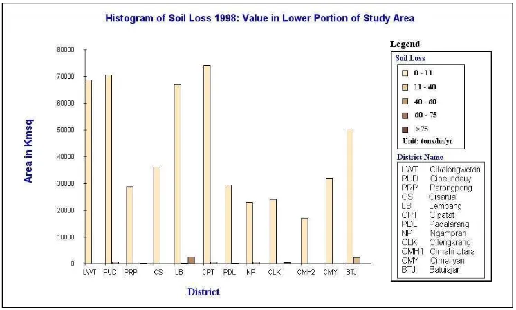
Fig (4.7): The total soil lo ss area in (km square) in each district in lower potion ...67
Fig (4.8): The soil loss rate in each district in lower potion...68
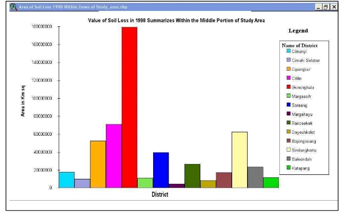
Fig (4.10): The soil loss rate by erosion in middle portion...69
Fig (4.11): The total soil loss area in (km square) due to erosion ...69
Fig (4.12): The total soil loss area in (km square) by erosion of each district ...70
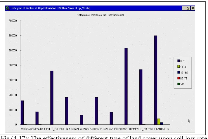
Fig (4.13): The effectiveness of different type of land cover upon soil loss rate ...71
Fig (4.14): The soil loss in area amount in year 1998...71
Fig (4.15): The soil loss rate of Lower portion in year 1998...72
Fig (4.16): The soil loss in area amount based on year 1998 land cover type ...73
Fig (4.17): The soil loss in rate based on year 1998 land cover type...73
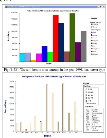
Fig (4.18): The soil loss in area amount in the year 1998 land cover type ...74
Fig (4.19): The soil loss rate in the year 1998 land cover type ...74
Fig (4.20): The land cover (C) factor effectiveness on erosion rate in 1993 ...75
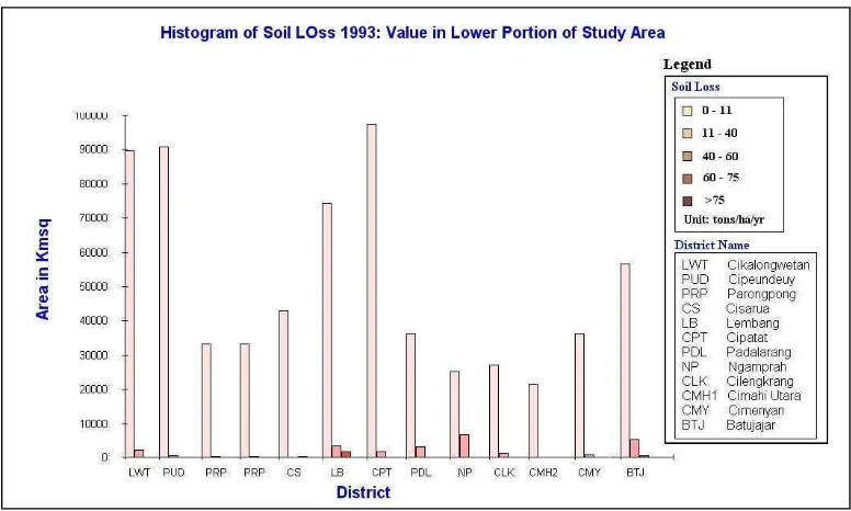
Fig (4.21): The soil loss area by erosion in lower portion of study area ...76
Fig (4.22): Soil loss rate in lower portion of study area...76
Fig (4.23): Soil loss rate in each district in year 1993...77
Fig (4.24): Soil loss rate in each district in year 1993...78
Fig (4.25): The soil loss rate in area by erosion in lower portion of study area...78
Fig (4.26): Soil loss rate amount in study area at 1993...79
TABLE (2.1): Data Layer And GIS Description For Rusle Factor ...20
Table (4.1): Name and History of Satellite Imagery for doing analysis ...43
Table (4.2): The Accuracy assessment of each class of land cover classification (2003) ...49
Table (4.3): The Physical Characteristics of the Soil Types in the Study Area...52
Table (4.4): The Classification of Soil Group in Hydrology based on Texture...54
Table (4.5): The Yearly Erosion Rate of Study Area by using RUSLE...65
LIST OF APPENDIX
APPENDIX-1: THE LOCATION OF WATER LEVEL GAUGE STATION IN UPPER CITARUM WATERS HED ...1
APPENDIX-2: RAINFALL EROSIVITY (R) FACTOR FOR BANDUNG REGENCY...2
APPENDIX-3: SOIL MONOGRAPH...3
APPENDIX-4 :THE SOIL ERODIBILITY(K FACTOR) OF BANDUNG REGENCY...4
APPENDIX-5: SLOPE LENGTH (LS) FACTOR MAP...5
APPENDIX-6: LAND COVER CLASSIFICATION OF BANDUNG REGENCY IN 2003 ...6
APPENDIX-7: LAND COVER CLASSIFICATION OF BANDUNG REGENCY IN 1998 ...7
APPENDIX-8: LAND COVER CLASSIFICATION MAP OF 1993...8
APPENDIX-9: LAND COVER CLASSIFICATION MAP OF 1989...9
APPENDIX-10: MAP LAYOUT OF EROSION POTENTIAL AREA (2003) ..10
APPENDIX-11: MAP LAYOUT OF ER OSION POTENTIAL AREA (1998) ..11
APPENDIX-12: MAP LAYOUT OF ER OSION POTENTIAL AREA (1993) ..12
APPENDIX-14: THE COMPARISON OF EROSION IN BANDUNG REGENCY BASED ON FOUR DIFFERENT LAND COVER SCENARIO ...14
APPENDIX-15: LAND DEGRADATION MANAGEMENT MAP ...15
APPENDIX-16: FACTOR C CLASSIFICATION VALUE...16
APPENDIX-17: P - FACTOR FOR SEVERAL CONSERVATION PRACTICES ...17
I. INTRODUCTION
1.1. Background
Erosion is the removal of surface material from the Earth's crust, primarily
soil and rock debris, and the transportation of the eroded materials by natural
agencies. It’s most important agent is moving water (Sposito, 1999). The concept
of multiple soil functions and competition is crucial in understanding current soil
protection problems and their multiple impacts on the environment. Soil erosion,
in particular, is regarded as one of the major and most widespread forms of land
degradation, and, as such, poses severe limitations to sustainable land use.
Soil erosion is a detrimental process both on-site and off-site. Soil erosion
not only reduces soil depth, but also reduces the capacity of soils to hold water
due to sealing, and depletes plant nutrients in the soil. This reduces soil
productivity and causes long term reduction in crop yields (Nanna, 1996), since
the necessary plant nutrients are washed away. It is estimated that annual crop
production becomes uneconomical on 20 million hectares of land in the world
(Elirehema, 2001). This raises concern about the ability of land to feed the
ever-increasing population. Moreover, soil erosion also creates off site environmental
problems, such as water pollution, silitation of reservoirs and degradation of
coastal ecosystems. It is thus necessary to understand where erosion is taking
place in order to design sound conservation measures (Kadupitiya, 2002a).
Soil losses due to erosion can be considered as irreversible in relation to
from less than 0.02 to more than 10 metric tons per hectare of soil lost annually,
rates of soil loss exceeding 10 metric tons per hectare annually occurrences of
accelerated erosion. It is important to note that this accelerated soil loss is
equivalent to less than 1 mm of soil depth, making erosion damage very difficult
to observe over short time spans (Sposito, 1999). Erosion is extremely costly for
developing countries. Besides the damage to infrastructure, fisheries, and
property, erosion of precious top soils costs tens of billions of dollars worldwide
each year.
Vegetation cover is a very crucial factor in reducing soil loss (Petter,
1992). In general, as the protective canopy of land cover increases, the erosion
hazard decreases (Mkhonta, 2000). It protects the soil against the action of falling
rain-drops, increases the degree of infiltration of water into the soil, maintains the
roughness of the soil surface, reduces the speed of the surface runoff, binds the
soil mechanically, diminishes micro-climatic fluctuations in the uppermost layers
of the soil, and improves the physical, chemical and biological properties of the
soil (Petter, 1992). As long as vegetation cover is unbroken, erosion and runoff
are small despite erosivity of the rainfall, slope steepness and soil instability. The
effects of vegetation cover on erosion processes especially on surface erosion are
varied depending on the type of vegetation cover, density, undergrowth cover and
litter. These determine the interception loss, absorption of kinetic energy and
increasing water infiltration. Land with good cover allows soil redundancy to
overland flow. Vegetation acts as a protective layer or buffer between the
atmosphere and the soil. The above ground cover absorbs energy of falling
ground components comprising the root system contribute to the mechanical
strength of the soil (Hagos, 1998).
Controlling erosion requires data on relative erosion rates, spatial extents,
vulnerable areas, current sources, relative contributions from different sources and
likely effects on land use (Meijerink and Lieshout, 1996). In many areas,
quantitative data on erosion rates is severely lacking (Nadeem, 1999). This data is
necessary for land management decisions in assigning priorities for erosion
control (Jack, 2002; Moore and Burch, 1986). It is financially impractical to have
conservation in all areas, rendering the need to identify and prioritize critical areas
(Wessels et al., 2001). Such information enables prevention of various forms of
degradation before they caused irreparable damage (Wessels et al., 2001).
Soil erosion modeling has proved to be a sound approach in generating
quantitative data (Shigeo et al., 1998). Models are effective predictive tools of soil
loss (Nearing et al., 1994). Models are particularly useful for evaluating the
impacts of intensified land use on soil loss, water quality and for evaluating the
potential effectiveness of mitigation or remedial measures before large sums of
money are invested in such measures (Moore and Burch, 1986).
Several studies (Shrestha, 1997; Shrestha, 2000; Wessels et al., 2001)
have shown that GIS is an excellent tool in erosion modeling. GIS modeling does
not only predict consequences of human actions on erosion, but it is also useful in
the conceptualization and interpretation of complex systems as it allows
decision-makers to easily view different scenarios. Most of the data used in models i.e.
first stage input to identify and map of degraded lands (Jaroslav et al., 1996;
Shigeo et al., 1998).
1.2. Identification
The island of Java is one of the most densely populated areas in the world.
A chain of volcanoes, some still active, have enriched the soil so that it is
generally very fertile. Since ancient times, Java has been a center of educational,
economic, cultural and political activity in Indonesia. Java has been until recently
the main producer of rice and sugar in the country. The fertile plain in the north of
the island is intensively cultivated throughout the year. To the south, fertile
agricultural lands have been developed in several river basins. If these are farmed
without conservation measures, the result is erosion and increased flooding.
However, because of the growing population has already occupied all
available land in the plains, people have invaded their agricultural purpose to
hilly and mountainous regions. For this reason, many reservoirs have been
constructed to manage water resources for irrigation and sanitation, as well as
hydroelectric power in west Java. About 60% of the population of Indonesia lives
in Java and Madura, and almost all of the land are being utilized for agriculture
(75%). With a population growth of 1.7% annually, the number of families that
depend upon agriculture will be increased by about 150,000 each year. This will
result in the conversion of forest land at a rate of 18,000 ha annually, with about
40,000 ha of agricultural land being converted each year into residential and
industrial purposes in west Java (World Bank 1990).
Because of the high population density, much of the land on west Java
conservation purposes has already been used for urbanization and agriculture.
Now only just over 6 million (hectare) of Java Island are covered with forest.
Because of population growth, these areas will undoubtedly continue to diminish.
The land currently within the forestry department boundary in west Java is about
22% or about 800,000 hectares less than the recommended area. Furthermore,
many of the designated forest lands are not in fact forested in the late 1980's, the
island of Java especially west Java ( Java Barat) was losing 770 million metric
tons of topsoil every year at an estimated cost of 1.5 million tons of rice, enough
to fulfill the needs of 11.5-15 million people. Only the West Java area (Jawa
Barat), the erosion rate per year is around 32,931.061 ton/th (1 juta truk tronton=
30 ton). (Source: BAPEDA 2002, DATA 2001/ RTRW Province Jawa Barat 2010,
Agro-ecological Analysis for Agricultural Development in Indonesia).
There are 13 watersheds in Java have which have critical erosion
problems. The Citarum watershed which is most important for electricity and
drinking water for Java Island is situated in west Java. The upper Citarum
watershed is now facing many environmental problems caused by the relatively
rapid population growth demanding change and development of new settlement
areas. The density of the population is relatively high: 1,640 people per km2.
There has been a 7-fold increase in silt load in the Citarum River over a
recent 3-year period. This is rapidly filling Indonesia's largest reservoir which
located downstream at Jatiluhur. For the whole Java, "Critical" lands outside of
covering forests include 5690 km2. Soil erosion rates are 990 to 4040 t/ km2/ year
and are increasing. Indonesia's main island of Java must be one of the most eroded
classifies more than 10,000 km2 (8% of croplands) as critically eroded. The land
is said to be so badly degraded that it is already, or soon will be, unable to sustain
even subsistence agriculture. Some small fields are losing 5 cm of soil/ year
(150,000 t/ km2/ year).(Source: The Earth's Carrying Capacity --Some
Literature Reviews, http://home.alltel.net/ bsundquist1/index.html available: 10
pm, 14 January, 2006).
Fig(1.1): The erosion assessment rate occurrence in west Java area
(Source: http://home.alltel.net/ bsundquist1/index.html)
The Bandung basin which is the main portion of upper Citarum watershed
seriously faces routine annual floods caused by an increase of erosion,
sedimentation and pollution problem. So that area needs to maintain
environmental condition for future uses.
This study will attempt to evaluate the impacts of different land use cover
types on soil loss by employing GIS based modeling techniques in order to
identify the effects of land degradation on its generation. Very light (0-15 Ton/ Ha/ yr)
Light (15-60 Ton/ Ha/ yr)
Intermediate (60-180 Ton/ Ha/ yr)
Critical (180-480 Ton/ Ha/ yr)
1.3. Objective
The objectives of this study are as follows:
• Estimation of soil erosion potential based on soil loss condition in the
study area.
• Examination of land cover change effect on soil erosion.
Output
• Soil erosion potential area using RUSLE.
• Correlation between land cover changed with potential soil erosion.
Benefit
• Provide the snapshot view of erosion potential assessment for decision
maker to implement the land use planning for declining land degradation
1.4. Thesis Structure
The thesis is divided into 5 chapters. The first chapter identifies the
research background, scope and objectives emphasizing on the need for this study.
Chapter two discusses the background on the theoretical aspects of erosion with
highlights on factors that influence it focusing on soils degradation problems.
Various methods of erosion modeling are briefly specified in this chapter and
finally a short description of the approaches employed in this study is given. In
chapter 3, a description of the study area is given mentioning among others
its location, climate, soil characteristics and geology. Moreover, Chapter 3
introduces the modeling approaches implemented in this study. It gives detailed
descriptions on the components used and specifies the data requirements of
each approach. Following this the activities involved in attaining the required data
used in preparing the input maps and the parameterization of the parameters
required is mentioned. The results of the study are presented in chapter 4. This
includes the results on the analysis of soil loss by erosion based on RUSLE and
the model predictions relating them to different land use/ cover types. Finally in
chapter 5, conclusions on the results of the study are made. Limitations of the
study are highlighted and some recommendations based on the study are given in
II.
LITERATURE REVIEW
2.1. Erosion
Soil erosion is one form of land degradation besides soil compaction, low
organic matter content, loss of soil structure, poor internal drainage, stalinization
and soil acidity problems. In particular, soil erosion is defined as: “physical
removal of topsoil by various agents, including falling raindrops, water flowing
over and through the soil profile, wind velocity and gravitational pull” (Lal 1990).
Historically, soil erosion began with the beginning of intensive agriculture
activities, where people are removing protective vegetation cover and growing
various food crops on disturbed soil surface.
In addition, some other large-scale opening of vegetation through
commercial logging, preparation of timber and crop estates, and expansion of
human settlement accelerated it. Nowadays, soil erosion is almost universally
recognized as serious threat to human’s well being. This is confirmed by facts of
active supports given by most governments to soil conservation programmes
(Hudson 1995). A general figure of rain erosion susceptibility is presented in
Fig (2.1): Distribution of rain erosion throughout the world (Hudson 1995)
Soil erosion caused by water is a serious problem in sub humid, semiarid,
and arid regions. Inadequate moisture and periodic droughts reduce the periods
when growing plants provide good soil cover and limit the quantities of plant
residue produced. Erosive rainstorms are not uncommon and they are usually
concentrated within the season- when cropland is least protected (Wischmeier and
Smith, 1978).
This energy in the form of rainfall causes splash erosion. The potential
energy for erosion is converted into kinetic energy, the energy of motion of the
running water. This kind of energy formed by runoff causes inters rill, rill, gully,
and riverbank erosion.
2.2. Factors Affecting Soil Erosion
Agents of erosion are the carriers or the transport system in the movement
of soil (e.g. water, wind). Factors of erosion are those natural or artificial
parameters that determine the magnitude of perturbation, e.g. climate, topography,
soil, vegetation and management. Erosion may not occur even when the agents
as farming practices, deforestation and cropping systems that facilitate the effects
of agents and factors of erosion and accelerate the various erosion processes
(Bergsma 1996; Lal 1990). The factors affecting soil erosion by water are:
2.2.1. Climatic Erosivity
Erosivity refers to the aggressively of the climate, or more precisely the
energy of such climatic elements to cause erosion. Climatic factors that affect
erosivity are precipitation, wind velocity, water balance, mean annual and
seasonal temperatures, etc.
2.2.2. Soil Erodibility
Erodibility is the susceptibility of soil to erosion. This is an inherent
property of the soil and is influenced by soil characteristics (e.g.) texture,
structure, permeability, organic matter content, clay minerals and contents of iron
and aluminum oxides.
2.2.3. Landforms
Erosion also affected the terrain relief through degree and length of slope,
shape of slope and slope aspect. In general, the higher the slope gradient, the more
soil erosion by water occurs.
2.2.4. Human
Human activities affect soil erosion through their measures to natural
resources. Human activities related to erosion are deforestation, grazing, faulty
farming system and cropping intensity. However, some activities in terms of soil
conservation measures are reducing the amount of soil erosion (e.g. contouring
2.3. Land degradation and land use/ land cover change
Land use and land cover change have become a central component in
current strategies for managing natural resources and monitoring environmental
change. Since the late 1960’s, the rapid development of the concept of vegetation
mapping has lead to increased studies of land use and land cover change
worldwide. Providing an accurate assessment of the extent and health of the
world’s forest, grassland, and agricultural resources has become an important
priority.
2.3.1. Land use and land cover
Every parcel of land on the Earth’s surface is unique in the cover it
possesses. Land use and land cover are distinct yet closely linked characteristics
of the Earth’s surface. Land use is the manner in which human beings employ the
land and its resources. Examples of land use include agriculture, urban
development, grazing, logging, and mining. In contrast, land cover describes the
physical state of the land surface. Land cover categories include cropland, forests,
wetlands, pasture, roads, and urban areas. The term land cover originally referred
to the kind and state of vegetation, such as forest or grass cover, but it has
broadened in subsequent usage to include human structures such as buildings or
pavement and other aspects of the natural environment, such as soil type,
biodiversity, and surface and groundwater. (Myers, 1988)
Land use change is generally conscious, volitional responses by humans or
human societies to changes in biophysical or societal conditions. It is a response
indicator, therefore, reflecting how and to what extent society is responding to
conditions. This does not exclude the possibility that some land use changes may,
in turn, constitute a driving force for changes in the state of the environment. That
is in the very nature of the complex causal network (not a simple causal chain),
including a number of feedback loops, that is society's relationship with its
environment.
As is the case for land use change, it is doubtful whether a single or
aggregate measure of land condition change would be feasible. What is feasible in
principle is an estimation of the change in the different land qualities that
influence the suitability of the land for one use or another, or for conservation
purpose, for example, of biodiversity and erosion for land degradation. (Land
qualities are discussed in FAO, 1976).
2.4. GIS and RS in Soil Erosion Modeling and Land Use/Cover Change
Soil erosion is spatial phenomena, thus geo-information techniques play an
important role in erosion modeling (Yazidhi, 2003). While this is agreeable, the
quality of the results matches the quality of the input data used (Svorin, 2003).
Land use data required to run erosion model can be derived from remotely sensed
data. In a GIS environment it is possible to link data generated from remote
sensing with their spatial location (Mkhonta, 2000). In general, the use of
geo-information techniques offers the following advantages in erosion modeling:
(i) fast and cost effective estimates,
(ii) possibilities to investigate larger areas,
(iii) greater possibilities of continuous monitoring of these areas and
(iv) possibilities to refine the soil erosion model depending on the required
According to Yazidhi (2003), the use of digital elevation models and GIS
offers possibilities to estimate more relevant topographical parameters that are
useful in soil erosion modeling.
2.4.1. Land Cover Mapping
Land cover mapping is one of the most important and typical applications
of remote sensing data. Land cover corresponding to the physical condition of
ground surface, for example, forest, glass land etc., while land use reflects human
activities such as the use of the land, for example, industrial zone, residential
zone, agricultural fields etc.
To prepare, the land cover mapping from digital images “land cover
classification” should be done. There are two kinds of classification, i.e.
supervised and unsupervised classification.
2.4.2. Supervised Classification
Supervised classification is the method used to transform multi spectral
image data into thematic information classes. This procedure typically assumes
that imagery of a specific geographic is gathered in multiple regions of the
electromagnetic spectrum.
In supervised classification, the identifying and location of feature classes
or cover types (urban, forest, water, etc) are known beforehand through fieldwork,
analysis of aerial photographs, or other means. Typically, identify specific areas
on the multispectral imagery that represent the desire known feature types, and
use the spectral characteristics of theses known areas to train the classification
program to assign each pixel in the image to one of these classes. Multivariate
are calculated for each training region, and each pixel is evaluated and assigned to
the class to which it has the most likelihood of being a member (according to rules
of the classification method chosen).
One of the sample classification strategies that may be used is Maximum
Livelihood Classifier. The maximum livelihood was adopted by using the training
samples of the landsat image and ground truth. Actually, this is one of the most
popular methods of classification in remote sensing, in which a pixel with the
maximum likelihood is classified into corresponding class.
2.5. Runoff Erosion Potential with GIS Based Spatial Analysis Model
Spatial Analysis extends the basic set of discrete map features of points,
lines and polygons to surfaces that represent continuous geographic space as a set
of contiguous grid cells. The consistency of this grid-based structuring provides a
wealth of new analytical tools for characterizing “contextual spatial
relationships”, such as effective distance, optimal paths, visual connectivity and
micro-terrain analysis. In addition, it provides a mathematical/statistical
framework by numerically representing geographic space.
Spatial Statistics, on the other hand, extends traditional statistics on two
fronts. First, it seeks to map the variation in a data set to show where unusual
responses occur, instead of focusing on a single typical response. Secondly, it can
uncover “numerical spatial relationships” within and among mapped data layers.
The model assumes that erosion potential is primarily a function of terrain
steepness and water flow. Then the result is combined with the human factor.
Admittedly the model is simplistic but serves as a good starting point for a spatial
Fig (3.1): The general information of runoff erosion model based on spatial analysis
2.6. Hybrid Erosion Modeling Approach
Empirical models which is one of statistical model, describe erosion using
statistically significant relationships between assumed important variables where a
reasonable database exists (Kadupitiya, 2002a). Empirical models are based on
defining important factors through field observation, measurement,
experimentation and statistical techniques relating erosion factors to soil loss
(Petter, 1992). In empirical models, the inherent processes involved are not used
and the models can only be operated in the designed direction where inputs go
into one side of the equation and the out put on the other side. Empirical models
are quick in predicting erosion, but are site specific and require long-term data
(Elirehema, 2001). Most models used in soil erosion studies are empirical models.
The most widely used empirical model is the Universal Soil Lose Equation
Universal Soil Loss Equation (RUSLE) and Modified Universal Soil Loss
Equation (MUSLE) etc, which are based on modifications made on USLE. The
GIS can also be used as a controlling tool for application ranges of model
parameters, especially the digital elevation model (DEM) related topographic
variables used in erosion modeling.
2.6.1. Revised Universal Soil Loss Equation: RUSLE
The Revised Universal Soil Loss Equation is being developed by the
USDA's Agricultural Research Service. The model will be refined and improve
the accuracy of the original Universal Soil Loss Equation (USLE) to estimate the
effects of various conservation systems on soil erosion.
(i) Model and Components
The RUSLE is an empirical equation that predicts annual erosion
(tons/ha/yr) resulting from sheet and rill erosion in croplands. The USLE is
factor-based, which means that a series of factors, each quantifying one or more
processes and their interactions, are combined to yield an overall estimate of soil
loss. It is the official tool used for conservation planning in the US and many
other countries have also adapted the equation. The equation is:
A = R * K * L * S* C* P
where,
A = Annual soil loss (tons/hectare/yr) resulting from sheet and rill
erosion. This is the predicted value resulting from the execution
of the equation above.
This factor measures the effect of rainfall on erosion. The R
factor is a summation of the various properties of rainfall
including intensity, duration, size etc. It is computed using the
rainfall energy and the maximum 30 minutes intensity (EI30)
K= Soil erodibility factor.
The soil erodibility factor measures the resistance of the soil to
detachment and transportation by raindrop impact and surface
runoff. Soil erodibility is a function of the inherent soil
properties, including organic matter content, particle size,
permeability, etc. Because these properties vary within a given
soil, erodibility (K values) also varies.
L= Slope length factor.
This factor accounts for the effects of slope length on the rate of
erosion.
S = Slope steepness factor.
This factor accounts for the effects of slope angle on erosion
rates. All things being equal, higher slope values have greater
erosion rates.
C = Cover management factor.
Accounts for the influence of soil and cover management, such
as tillage practices, cropping types, crop rotation, fallow, etc...,
on soil erosion rates.
Accounts for the influence of support practices such as
contouring, strip cropping, terracing, etc...
Once these factors have been determined for a field of interest A can be computed.
Also, the equation can be used to determine the desired cover management factor
(C) or erosion control (P) if the allowable soil erosion rates are known. Thus, in
this research use the RUSLE to simulate the impact of changes in land use and
land cover on soil erosion, anthropogenic impacts on the environment.
Table (2.1): Data Layer and GIS Description for RUSLE Factor
Erosion databases,
factors
Data layers Description of GIS procedures (include cross-references)
Erosivity (R) Rainfall data
Spatial interpolation of station EI values; stored as R-
factor map.
Erodibility
(K) Soil data
Assignment of numerical K-values to soil units by
reclassification of the soil unit polygon map with the K-
value column from the soil attribute table; stored as
K-factor map. Combining slope length and gradient (LS) Geomorphic
If regional geomorphologic relief classes exist, combined
LS-gradient or terrain factor values can be obtained using
a 2-Dim table with row wise, relief steepness classes and
column wise the slope length classes, resulting directly in
LS-value distribution for the area; stored as an LS-map
file.
Land Cover Land cover, Farm dbs
If necessary pre-processing or spectral classification of
remote sensing data; assignment of C-factor values to land
cover RS data classes using cover attribute table; stored as
C- factor map;
Conservation
Practice
Farm
Land cover
For land use types with soil conservation practices,
reclassify C-factor map with P-factor values of land cover
2.6.2. Difference between RUSLE and USLE
The USLE (Wishmeier and Smith, 1978) is the most widely used model in
predicting soil erosion. It is used in education and research as a starting point in
developing understanding of erosion hazard prediction because of its simplicity
and clarity (Hagos, 1998). Many scientists have proposed changes, but all are
woven around the same concept of rainfall erosivity, soil erodibility, slope length,
slope class, land cover and land management factors are taken as directly
proportional to the rate of annual soil erosion (Sohan and Lal, 2001).
RUSLE is a revised version of USLE, intended to provide more accurate
estimates of erosion (Renard et al., 1994). It contains the same factors as USLE,
but all equations used to obtain factor values have been revised. It updates the
content and incorporates new material that has been available informally or from
scattered research reports and professional journals. The major revisions occur in
the C, P, and LS factors. The cover factor (C) and management factor (P) in
RUSLE consider not only agricultural land but also multifunctional land use type
and management. The slope length and aspect gradient factor combine to become
slope length and steepness factor (LS) in RUSLE.
2.7. High Conservation Value Forest (HCVF)
One of the Forest Stewardship Council (FSC) principles is the
management of High Conservation Value Forest (HCVF). This is relatively a new
principle, which has been developed to replace the previously used concept of old
growth or virgin forest. Through this principle, FSC requires unique approach in
managing forest ecosystem and conserving the biodiversity value (FSC 2001). In
preserve it. The key of HCVF principle is the concept of conservation values.
HCVF have nine principles.
The use of remote sensing and spatial information to support identification
of HCVF is certainly potential. Some of the HCVF elements could be assessed
through the remote sensing and GIS analysis resulting the location of forest area
containing some High Conservation Values (HCV). One HCV element, which is
potentially assessed by the support of remote sensing and GIS is HCVF principle
four. The principle four (HCVF 4) mention that “Forest areas which provide basic
services of nature in critical situations (e.g. watershed protection, erosion
control)”. That principle including (3) sub – factors, i.e.
• Functions as unique source of drinking water for local communities (HCV 4.1)
• Part of critical major catchments (HCV 4.2)
• Has critical erosion risk (HCV 4.3)
Ancillary data that can be used are topographic information and its derived
products (DEM, slope map and other terrain features to support prediction of
potential soil erosion risk (after Rainforest Alliance and ProForest 2003).
2.8. Accuracy of Modeling in GIS Environment
Accuracy is the degree of likelihood that the information provided is
correct. This definition focuses on two components of accuracy. The first and
more familiar aspect of accuracy is that it predicts the proportion of information
that is expected to be correct or the magnitude of error to be expected. The second
and often ignored aspect of accuracy is that it involves a probability. When a map
or other data set is asserted to be 80% accurate it means that when the data set is
The measure of this probability of having a higher or lower accuracy than
expected is termed the level of confidence. So, when a map is rated 80% accurate
with a 90% level of confidence it means that if a large number of accuracy tests
were done on the map, then 80% or more of the test points would be correct in 9
out of every 10 tests. The level of accuracy depends on the information to be
provided and the level of detail required. An acceptable level of accuracy is that
level where the costs of making the wrong decision are equal to the costs of
acquiring more accurate information.
In the GIS environment, map accuracy depends on many factors. At the
micro level, there are components such as positional accuracy, attribute accuracy,
logical consistency, and resolution. At the macro level, there are components such
as completeness, time, and lineage. Finally usage components are accessibility
and direct or indirect costs. There are also different sources of errors associated
with all geographic information. Some of the more common errors are related to
data collection, data input, data storage, data manipulation, data output, and the
way of using and understanding results.
Paper data such as different maps and associated geographic attributes and
data are used as one of the sources of input data to the GIS environment. In this
process the paper data are converted to digital data. The level of accuracy of the
digital data will be the same as paper data if they are correctly converted to the
digital form with a suitable package in an acceptable resolution. Once the data are
converted, the accuracy of the output data resulting from different manipulations
depends on the resolution power of the software done with the skill of the
2.9. Validation of soil erosion models
Model validation involves a procedure to determine how best the model
predicts soil loss rates in the real world. Traditionally validation of soil erosion
models has been implemented through the comparison of model output and
III. RESEARCH METHODOLOGY
3.1. Physical Condition of the Study Area
3.1.1. Location
The Bandung regency which include major portion in the catchments area
of the Saguling Reservoir is so called Bandung basin (Indonesia), with an area
approximately 2,283 square km2, geographically located between 6° 4' S to 7° 10'
S and 107° 15' E to 107° 45' E. The Bandung regency include (40) districts. For
doing sensitivity analysis, the study area need to make zone into three portions,
i.e. upper, middle and lower portion. Upper portion of study area consist of (12)
districts and middle and lower portion of study area consist of (14)
sub-districts. The detail list of sub-district which include in each portion was mention
in Appendix (18).
The topography of the Bandung basin in Bandung regency various from
flat to mountainous with a height from 650 meter to 2,000 meter above sea level.
And also the slope varies from gentle to very steep.
3.1.2. Climate
The study area has tropical climate under the influence of monsoon wind
as the same as other places in Indonesia. There are two seasons in this area, rainy
and dry season. The rainy season occurs from October until April, whereas the dry
season is taken place from June till October. The period from May till June can be
considered as transition period. Average rainfall in the surrounding area is
between 1,782 millimeter to 3,426 millimeter, for 30 years under consideration,
3.1.3. Geology and Geomorphology
The Land Mapping Units comprised: (1) flood plains, (2)
alluvio-lacustrine plains, (3) colluvial plains, (4) volcanic plains, (5) alluvio-volcanic fan,
(6) volcanic fans, (7) volcanic foot-slopes, (8) lower volcanic ridges, (9) middle
volcanic ridges, (10) upper volcanic ridges, (11) hills, and (12) mountains.
In general the Lithology of the upper portion of the study area which is the
location of Cikapundung catchment, consists of volcanic rock which has been
resulted from eruption of Tangkuban Perahu mountain.
According to Silitonga (1973), the study area consists of four units as
fallows:
1. The differentiated rock unit coming from the old sunda volcano comprises
volcano breccia, lahar and lava alternately.
2. The differentiated rock coming from the Tangkuban Perahu eruptions,
comprises sandy tuff, lapilly and breccia, lava and conglomerate.
3. Tuff pumice which came from Tangkuban Perahu eruption phase A,
comprises sandy tuff, lapilly, bombs, halloured lava, solid andest and
fractions of pumice
4. Lava which consist of basalt and gastubes, coming from the lava flows of
the Tangkuban Perahu.
The catchments can be divided into two main geomorphologic units, which
are volcanic origin and structural origin. Volcanic origin can be divided into four
sub units, which are volcanic cone, volcanic middle slope, volcanic lower slope
parts; northern and western part, separated by an east-west running normal fault
(Lembang fault).
Indonesia Map
Fig (3.1): The location of study area
3.1.4. Time
The study will be conducted from February 2006 up to May 2006.
3.2. Materials and Tools Requirement
The following materials are needed:
(1) Digital Topography maps at scale of 1:25,000
(2) Soil classification map at scale 1:250,000
[image:38.612.140.494.121.474.2](4) Satellite image: Landsat TM+ for four different years (1989, 1993, 1998
and 2003)
(5) Time series rainfall data
(6) Rainfall isohyetal map
3.2.1. Data Source
The materials that were used in this project divided into two types, which
are: primary data or field data and secondary data. The secondary data include soil
survey data, (10) years rainfall data and discharge data of at least two rainfall
stations in the study area. The spatial data raster format are soil type classification
map (1:25,000 scale), soil depth classification, slope length and isohyetal map of
the study area. The primary data consist of landset TM image and topographic
map. The rainfall intensity data and discharge data are provided by Agro-climate
and Hydrology research center, Ciomas, Bogor.
3.2.2. Tools
Hardware required minimum computer device: Intel Based PC or compatible
machine with Pentium IV processor.
Software required: ER Mapper 6.4 for Landsat TM image processing, ArcView
GIS 3.3 and Spatial Analyst Extension, Digital Elevation Model Extension, Soil
and water assessment tool extension and Hydrology modeling extension is
recommended for analysis the data, Microsoft excel 2003 for meteorological data
processing and Microsoft words 2003 for preparing the report. Moreover,
3.3. Procedure of application
In this study, an estimation of land degradation in the study area was
carried out based on the flowchart of the procedure to obtain the purpose of the
study. Literature Review Problem identification Research objective Data collection Primary Data Secondary data Land use and vegetative cover data Soil profile description Soil erodibility factor (K) Land cover management factor (C) Soil conservation factor (P) Climate data Topographic map Rainfall runoff erosivity (R) Rainfall data Contour line map Elevation (DEM)
Slope length & Slope steepness
factor (LS)
Preparation of map layers
Calculate erosion potential parameter
RUSLE erosion model
Land Degradation based on erosion
potential
Soil Survey
Data
1989,1993 Landsat TM+, 1998 and 2003 Landsat ETM+, Using Supervised and Unsupervised Classification for testing land use and cover change
Statistical analysis of land use and cover
change Given weight based on land used / cover
characteristic
3.4. Deriving Digital Elevation Model (DEM)
Digital Elevation Model (DEM) is an essential intermediate product that
was derived in this study. DEM is used as main input in calculating slope length
and slope steepness for prediction of potential erosion risk. In this study, a Digital
Elevation Model was derived from contour line map with original scale of
1:25.000 and contour interval 12.5 meter. The general process of deriving the
DEM is presented in figure (3.3). The contour line map was digitized and stored
in format of ESRI PC Arc/Info® line coverage. Since the elevation interpolation
algorithm requires point map as the input, the contour line map was converted into
grid (which have same grid cell size with desired DEM grid cell) and then
converted into point coverage. After the conversion was done, spline point
interpolation of ArcView® was carried out to produce elevation grid with
resolution of 30 metres. Nevertheless, the grid size of 30 meter was chosen to
have more detailed result and to have the same grid cell size with other spatial
3.5. Classified the Digital Image
Classification of remotely sensed data used to assign corresponding level
with respect to group with homogenous characteristics with the aim of
discriminating multiple objects from each other within the image.
Classification will be executed on the based of spectral or spectrally
defined features, such as density, textured in the future space. Its can be said that
classification divides the features space into several classes based on the decision
rule. Classification will be done according to fallowing procedure:
Step1: Definition of classification classes
Depending on the objective and the characteristics of image data, the
classification classes should be clearly defined.
Step2: Selection of feature
Features to discriminate selected classes should be established using
multi-spectral characteristics or features.
Step3: Sampling of training data
Training data should be sampled in order to determined appropriate
decision rules. Classification technique such as supervised or unsupervised
learning will then be selected on the basis of the training datasets.
Step4: Estimation of universal data sets
Various classification techniques will be compared with the training data,
Step5: Classification
Depending up on the decision rule, all pixels are classified in the single
class. There are two methods of pixel by pixel classification and pre-field
classification, with respect to segmented areas.
Popular techniques are as fallowed:
• Multi-level slice classifier
• Minimum distance classifier
• Maximum likelihood classifier
• Other classifier such as fuzzy set theory and expert system
Step6: Verification result
The classified result should be checked and verified for their accuracy and
reliability.
3.5.1. Supervised Classification
In order to classify a decision rule for classification, it is necessary to
know the spectral characteristics of features with respect to the population of each
class. The spectral features can be measured using ground based spectrometers.
However due to atmospheric effects, direct used of spectral effect is not always
available. For this reason, sampling of training data from clearly identified
training areas, corresponding to define classes is usually made for estimating the
population statistics. This is called supervised classification. Statistically unbiased
sampling of training data should be made in order to represent the population
correctly.
In this classification the user plays a primary role; based on ground data,
decision space of the different classes. For each category, has a number of field
locations throughout the study area has been determined on the ETM imagery.
The maximum likelihood classifier was used. Since there is a considerable
spectral difference between soil and vegetation on the image, classification for
erosion hazard was possible.
3.6. Preparation for RUSLE Model
To spatially estimate the potential erosion risk, distribution of rainfall
intensity, slope length and slope steepness factor derived from Digital Elevation
Model (DEM), soil map and land cover map were used to establish a map of
potential erosion risk. A revised universal model developed by USDA-ARS,
Revised Universal Soil Loss Equation (RUSLE) (Wischmeier & Smith in 1978) is
used to estimate the erosion risk of the study area, with the following equation:
A = R x K x LS x C x P
• R = Rainfall erosivity
• K = Soil erodibility
• LS = Topographic Factors
• C = Cover management
• P = Land Conservation
• A=Rate of erosion at certain area
Landset TM+ Geometric correction / Georeferencing Radiometric correction (Haze removal) Supervised
Classification Land Cover Map
Information erosion management practice Land Conservation Value Land conservation value map Cover Management Factor (C) Rainfall Intensity distribution
Calculate rainfall erosivity (R) Rainfall Intensity Map
Soil Classification
Map Calculate Soil erodibility (k)
Soil Erodibility Map (K factor) Rainfall Intensity distribution DEM (Raster)
Contour Line Map (12.5 interva)
TIN (Grid Coverage)
Interpolation Slope in % Slope Aspect
Topographic Map (LS factor)
Calculate with Map Calculator (A= R K LS C P)
Erosion Potential
Fig (3.4): The flow chart of prediction erosion process by RUSLE model
3.6.1. Rainfall-runoff Erosivity Factor (R)
The R factor represents the erosivity of the rainfall at a particular location.
Rainfall Erosivity (R) is originally calculated as a product of storm kinetic energy
(E) and the maximum 30-minute storm depth (I 30) summed for all storms in a
year. An average annual value of R is determined from historical weather records
and is the average annual sum of the erosivity of individual storms (Weischmeier
and Smith 1978). Regarding the study area, available dataset are records of
monthly rainfall amount (mm/month) and raindays (days/month), as well as an
isohyets map representing the general distribution of annual rainfall. As common
situation found in developing countries, there was no rainfall intensity data
derived for tropical areas (El-Swaify et al. 1985), was used to calculate R-Factor
based on annual rainfall amount.
R = 38.5 + 0.35P
Where R: annual rainfall-runoff erosivity factor (MJ.mm.ha-1.h-1.yr-1)
P: annual rainfall amount (mm) summed from monthly-recorded
rainfall amount (mm)
P value was derived from averaged annual rainfall record collected from
two rain station. Considering the spatial variation of the rainfall amount, the
isohyets map, with additional data from the rain stations, was interpolated to grid
map with 300 meter cell size to come up with spatial distribution of annual
rainfall. The grid map of annual rainfall was resample to 30 meters to allow
spatial overlay with grid map of other factors of RUSLE. All climatic data were
collected from BAHL (Agro-climate and Hydrology Laboratory).
3.6.2. Soil Erodibility Factor (K)
The soil erodibility factor is the average long-term soil and soil profile
response to the erosive power of rainfall and runoff. Soil erodibility factor
represents the effect of soil properties and soil profile characteristics on soil loss.
To determine the K-value for each soil type, the following equation was used
(Weischmeier and Smith 1978), given the silt fraction does not exceed 70%.
Where:
K : Soil Erodibility Factor (t.ha-1.MJ-1.ha.mm-1.h)
OM : Organic matter content (%)
M : Product of primary particle size fractions
M = (% Silt + % Very Fine Sand) * (100 - % Clay)
(3.2)
S : Code of Soil Structure
P : Code of Soil Permeability
3.6.3. Slope Length and Slope Steepness Factor (LS)
Slope length (L) is defined as horizontal distance from the origin of
overland flow to the point where the slope gradient decreases considerably, so that
the deposition begins, or where runoff becomes concentrated in a defined channel
(Weischmeier and Smith 1978). Surface runoff will usually concentrate in less
than 400 ft, which is the recommended practical slope-length limit in RUSLE.
The LS factor is the most difficult one to derive in GIS, because the length
aspect is not direct. The digital elevation model (DEM) of the study area was used
in generating the LS factor. Because of the difficulties commonly experienced in
generating the LS factor, two methods were used. In the first method, the slope
steepness (S) and length (L) factor layers were generated separately and later
overlaid to get the RUSLE slope length factor layer (Mongkolsawat et al., 1994).
In the second method, an ArcView based technique was used. The LS
factor can be estimated from the DEM. The technique described for computing LS
requires a flow accumulation theme. Flow accumulation can be computed from a
DEM using the hydrologic extension or other watershed delineation techniques.
Flow accumulation is used to estimate slope length. First we will compute slope
steepness using the DEM. Before beginning the analysis, check the Analysis
Properties to make sure the extent and gird cell size are acceptable. The grid cell
size should be set to the grid cell size of the DEM for this analysis.
• Make the DEM active, select the Surface pull down menu as shown below
• Use the map calculator to create new themes of the flow accumulation
classification as 0 and 1.
• Use map calculator to compute the LS factor as shown below. Note that
the slope must be converted to radians from degrees by multiplying the
slope by 3.14 (pi) and dividing by 180.
The technique for estimating the RUSLE’s LS factor that will be used here
was proposed by Moore and Burch (1986a and 1986b). They derived an equation
for estimating LS based on flow accumulation and slope steepness. The equation
is:
LS = (Flow Accumulation * Cell Size/22.13)^0.4 * (sin slope/0.0896)^1.3
Fig (3.5): The process of manipulate LS factor from DEM
3.6.4. Cover Management Factor (C)
C factor reflects the effects of vegetation cover on soil erosion, hence, this
factor is often used to compare relative impacts of management options on
conservation plan. The land cover-management factor (C) is the most important in
RUSLE because it represents conditions that can easily be managed to reduce
erosion (Renard et al., 1994). The C factor reflects the effect of cropping and
management practices on erosion rates. It indicates how conservation affects the
average annual soil loss and how soil loss potential will be distributed during
cropping and other management schemes (Renard et al., 1997). It is based on the
concept of deviation from a standard plot under clean continuous fallow
cultivations. In RUSLE, C is computed from soil loss ratios (SLR) i.e. prior land
use (PLU), canopy cover (CC), surface cover (SC) and surface roughness (SR).
In this study, a land cover type map was produced as the result of image
classification of Landsat ETM+ Image. The C factor value can be ranked based on
the FAO standard tables (see Appendix-15) given information about land use and
management for land degradation assessment.
3.6.5. Land Conservation Factor (P)
The assign value of factor (P) as a attribute field according to FAO
standard value and rating. Put the value of P as 1 for non-conservative area and
zero for conservative forest area. For Agricultural area, the P factor classification
based on the agricultural practice, which is normally divided into: terraces
cropping, contour cropping, mulch cropping and permanent ground cover type.
The table showed the P- factor classification for several conservation practices in
Indonesia (Hammer, 1980) in Appendix-16.
3.6.6. Calculate the Erosion Rate
Using map calculator can estimate RUSLE soil erosion for every grid cell
in the area of interest.
3.7. Analysis the Model
In this research, propose to use analysis method with changed the
parameter “land use and land cover” differencing between four landsat TM
images of different dates to compare the rate of erosion by soil loss in each district
IV. RESULTS AND DISCUSSIONS
4.1. Land Cover Change Classification
The large areas of land cover are mapped at 1:50,000 scale using Landsat
TM and/or ETM data. The land cover mapping was carried out using the FAO
Land Cover Classification System (LCCS), a new methodology especially created
for land cover mapping and now used worldwide. The following list describes the
main phases applied in the present study, for the creation of the land cover maps:
1. Satellite data selection
2. Satellite data preprocessing
3. Satellite data classification
4. Satellite data interpretation and vectorization of the resulting units
5. LCCS classification
6. Field checking
7. Composition of final land cover maps
4.1.1. Satellite Data Selection
As previously indicated, all areas under study were used in July 1989 for a
rapid assessment of local physiographic and of the main land cover classes
occurring there. Satellite data were selected on the seasonal based of the crop
calendar for the main crops. Although the purpose of the study was to prepare
land cover maps and not crop inventories, it was considered of some importance
to be able to separate the crops in the field at the time of satellite data acquisition.
Consequently, an image acquired in December is included in the wet season,
based calendar of the satellite image, we can consider not only permanent land
cover changed by human factor but also temporal changed by season. The
information of images use in this research is shown in Table(4.1).
Table (4.1): Name and History of Satellite Imagery for doing analysis
Types of image Path row Date of acquisition Landsat ETM + T 1220650126034 122-065 December 6, 2003
Landsat ETM + T 1220650816982 122-065 August 16, 1998
Landsat ETM + T 1220650919932 122-065 September 19,1993
Landsat TM + T 1220650706892 122-065 July 6, 1989
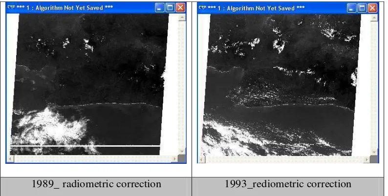
4.1.2. Satellite data Processing
This is the first step prior to the remotely sensed data to be analyzed for
removing some errors of satellite imagery. There are two common types of errors,
radiometric and geometric, in remotely sensed satellite image to perform for
enhancing quality of image for analysis. Fig (4.1) shows the process of image
preprocessing for analysis.
Fig (4.1): Flow Chart of Image Preprocessing
Raw Image
Radiometric Correction
Geometric Correction
Corrected Image
Image Calibration Atmospheric Correction
Ground Control Poi