Predictive functional control (PFC) for use in autopilot design.

(1)

The

University

Of

Sheffield.

Automatic

Control &

Systems

Engineering.

Predictive Functional Control (PFC)

For Use in Autopilot Design

By: Hyreil Anuar Kasdirin MSc in Control Systems: August 2006

Supervisor: Dr J A Rossiter

(2)

ABSTRACT

This paper discusses the design and implementation of PFC as a controller for an

autopilot missile. Two linear continuous time missile models which are derived from

nonlinear model produced by Horton [13] and another from the basic Ballistic Missile

[10] are used for the prediction models. The PFC algorithm is developed based on the

models. The PFC algorithm developed is seems intuitive and computationally simple as

the missile need not to be very complicated as it will explode as it reaches the target.

Furthermore, the analysis and issues of the implementation relating linear discrete-time

stable and unstable process are being discussed. In addition, PFC tuning parameters play

an important part of the autopilot controller. Thus, the result indicated that the PFC

control law is built better when choosing the dynamic pole of the missile mode to be the

desired time constant, 'P and small coincidence horizon n1 as performing in single

coincidence point. The implementation of PFC on the missiles-scenario is also developed

for Model Missile I and 2. As a result, some positive results is illustrated and discussed

as the both missile followed its reference trajectory during simulation using MATLAB

7.0.

Keywords: Predictive Functional Control (PFC), autopilot design, discrete-time

state-space models

(3)

EXECUTIVE SUMMARY

Introduction/Background

This paper will concentrate on the basic handling of PFC as a controller for autopilot

missile. The formulation of PFC will be developed as well as how PFC handles with

stable and unstable process. A particular type of missile and onboard guidance system has

not been specified in the reference missile model. However, the paper briefly explained

some missile models and its missile guidance control. Thus, the result and

implementation of the PFC algorithm as a controller of autopilot missile will be further

discussed later on.

Aims and Objectives

The main aim of this project is to understand the design the PFC as a controller for an

autopilot missile. The principle objectives of this project are to understand and develop

the basic of PFC methodology. It also intended to analyze issues relating stable and

unstable process on PFC algorithm. Lastly, the objectives of this paper are to analyze the

results from the design and tests using PFC algorithm on missile models using MATLAB

7. 0 environment.

Achievements

At the end of this project the implementation of PFC is discussed. This paper will

concern on linear continuous-time stable and unstable missile model that only concern on

the aerodynamic control of the missiles. Furthermore, this paper shows that PFC is

developed successfully with one coincidence point, n 1• The tuning parameters of the PFC

algorithm; which are the desired time constant, 'I' and the control horizon, n are being

manipulated in order to give the best performance of the controller. As a result, it is

clearly illustrates that it is best to chose the dynamic pole of the missile mode to be the

desired time constant, 'I' and small coincidence horizon n1 as performing in single

coincidence point. This section also has successfully implementing PFC on unstable

(4)

before implementing Closed-Loop Prediction (CLP) on the modified PFC control law to

give stable and good response and performance. The implementation of PFC on the

missile-scenario is also illustrated by showing the result of discrete linear missile model 1

and 2. The section 4.5 clearly showing that PFC perform well as a missile autopilot

controller as it gave good trajectory as the reference trajectory moved and tum in

different direction. As a result, some problems faced and suggestions are also being

discussed.

Conclusion I Recommendations

At the end of this project it was recommended to improve the missile model as the

prediction model and develop the scenario of missile-target to see whether the PFC could

be used as a controller for the autopilot missile. In all, based on the achievement/result

the implementation of PFC algorithm seems intuitive and computationally simple. This

truly important as the missile controller need not to be very complicated as it will explode as it reaches the target.

ACS6200: Predictive Functional Control (PFC)

(5)

ACKNOWLEDGEMENT

I thank God Al-Mighty for giving me the opportunity to achieve my goal.

Here, I would like to express my gratitude and acknowledgement to Dr J. A. Rossiter for his guidance and continuous encouragement as well as motivation throughout the project.

I also would like to express my gratitude to my lovely wife and daughter for their

understanding, patience and moral support.

I would like to thank to the Kolej Universiti Teknikal Kebangsaan Malaysia (KUTKM),

for their financial support of this course. Last but not least, many thank to my family,

friends and all of the lecturers of The Department of Automatic Control and Systems, for

continuous support and encouragement to my study at the University of Sheffield, United

Kingdom.

HYREIL ANUAR KASDIRIN

(6)

LIST OF FIGURES

Figure 1.1 : Pitch, Yaw and Roll of a Missile ... . ... . ... ... .. .. .. ... .... 10

Figure 2.1 Basic structure of MPC .. ... ... .. ... .. .. .. .. .. . ... .. ... ... ... .. . .. .. .. ... .. 14

Figure 3 .1: The Airframe of Basic Missile . . . .. 26

Figure 3.2: Ballistic missile axis system. . ... ... ... .. .. .... ... 31

Figure 3.3: Sketch of an aerodynamic missile and axis system .... ... .. .. .... . .... . ... ... ... 34

Figure 3.4: Basic Layer of Automatic Missile Control .. .. ... ... .. ... 34

Figure 4.1: The Control and Output Response for Example 1 . . . 39

Figure 4.2: The Closed-loop Step Response for 'I'= 0.3 .. ... ... . ... 41

Figure 4.3 : The Closed-loop Step Response for 'I'= 0.6 ... ... ... .. ... . ... 42

Figure 4.4: The Closed-loop Step Response for 'I'= 0.9 ... .. ... ... .. ... ... 43

Figure 4.5: The Controller Response of Example 1 for 'I' = 0.94 .... . ... ... .. ... .. ... 46

Figure 4.6: The Root Locus and Bode Diagram for Missile Model 2 ... ... .. ... 47

Figure 4.7: The Controller Response of Example 1for'I'=0.94 ... ... .. .. .... ... ... ... 50

Figure 4.8: Sketch of an aerodynamic missile of Missile Model 1 Figure 4.9: The Missile Controller Response of Missile Model 1 Figure 4.10: Sketch of an aerodynamic missile of Missile Model 2 Figure 4.11: The Missile Controller Response of Missile Model 2 ... ... .. .. .. .. . ... ... .. .... ... 52

.. ... ... .. ... ... . 53

.... . .... .. ... ... . ... 55

(10)

[image:10.507.18.474.62.661.2]

LIST OF TABLES

Table 3 .1: The Motion Variables of the Basic Missile Model ... 27

Table 3.2: The Characteristics and the coefficients of Horton Missile Model 1

Table 3.3: Characteristics and coefficient of basic ballistic Missile Model 2

.. ... .... .. . 29

... .. ... 32

Table 4.1: Parameters of Example 1 .. ... ... .. .... ... ... ... 38

Table 4.2: Parameters Used for Tuning Parameters of PFC Algorithm of Example 1

Table 4.3: Parameters Used for Developed of PFC control law for Missile Model 1

Table 4.4: Parameters Used for Developed of PFC control law for Missile Model 2

ACS6200: Predictive Functional Control (PFq For Use in Autopilot Design

40

52

56

(11)

SECTION 1: BACKGROUND PROJECT

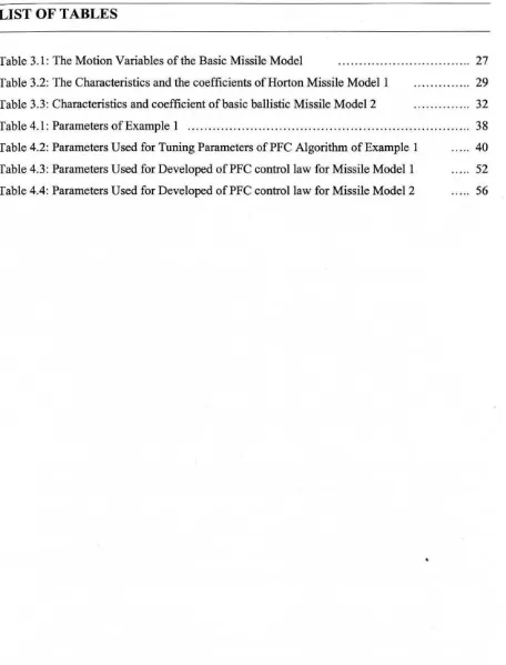
1.1 An Autopilot Missile

A missile is a projectile, often self propelled, which delivers a payload to a target.

Missiles have various launch platforms, ranges, targets, payloads and are typically guided

either remotely or automatically. Basically, there are 6 degrees of freedom which need to

be controlled. These angles are conventionally called yaw, pitch and roll (refer Figure

1.1) which all of these measures by the on-board sensors. In this paper, there are two

models that have been selected and they are only two degree of freedom.

Figure 1.1: Pitch, Yaw and Roll of a Missile

In this paper, the main point of research is the autopilot system of the missile. An

autopilot is a mechanical, electrical or hydraulic system used to guide a vehicle without

assistance from human being. Missile autopilot system is one of the examples of an

autopilot system. The main purpose of the autopilot missile is to enable the missile to

accomplish their mission autonomously, without any (or with minimal) input from the

missile operator. It includes the missile automated take-off or target hit, depends on its mission.

Nowadays, modern autopilot missiles use computer software to control the missile. It

uses the missile state information provided by the on-board sensors to drive the control

[image:11.505.24.464.58.484.2]

(12)

missile is also designed to hold certain parameters constant, for example its direction,

speed, altitude etc.

The control and guidance system is the brain of the autopilot missile. The on-board

control circuit need not to be too complicated or big as its mission is only target-hit

approach. Numerous missile designers and researcher have attempted to build effective

control of an autopilot missile such as using H-infinity controller [14] and Adaptive

controller [15] . In addition, this paper is continuing the work of Ben [16] and Nick [17] for implementing Model Predictive Control as a controller for autopilot missile. They have

successfully developed missile model and simulation of target-hit of the model. However,

they only concentrate briefly on the control section using Model Predictive Control (MPC).

Hence, this paper will only concern of the missile autopilot controller using Predictive

Functional Control (PFC).

1.2 Predictive Functional Control (PFC)

Predictive Functional Control (PFC), which developed by Richalet [1] is one of Model

Predictive Control (MPC) techniques that have been developed as a powerful algorithm

for controlling process plants. In this paper, the focus is on the implementation of the predictive functional control (PFC) on the missile dynamic models. PFC is based on the

same approach with all MPC strategies i.e., prediction of the future outputs, and

calculation of the manipulated variables for an optimal control. Therefore, PFC is also

based on the same principles which are using an internal model, specification of a

reference trajectory and determination of the control law.

1.3 Thesis Scenario: PFC as a controller of Autopilot Missile

This paper will concentrate on the basic handling of PFC as a controller for autopilot

missile. The formulation of PFC will be developed as well as how PFC handles with

stable and unstable process. A particular type of missile and onboard guidance system has

not been specified in the reference missile model. However, the paper briefly explained

some missile models and its missile guidance control. Thus, the result and

(13)

implementation of the PFC algorithm as a controller of autopilot missile will be further

discussed later on.

1.4 Aims and Objectives

Therefore, regarding the thesis scenario of this project, the aim of this project is as

follows:

• Understand the design the PFC as a controller for an autopilot missile.

In addition, the objectives of this project are to:

• Understand and develop the basic of PFC methodology.

• Analyze issues relating stable and unstable process on PFC algorithm.

• Analyze the results from the design and tests using PFC algorithm on missile

models using MATLAB 7.0 environment.

1.5 Chapter Outline

Based on the aim and objectives given above, this project is investigating the design an

autopilot control system of a guided missile using PFC controller.

The second section will be looked on some basic theory of PFC as a controller so that it

can be formulated and implemented in the following sections. However, at first, this

section will describe the basic of MPC algorithm and its optimal control that has become

an efficient control strategy for a large number of processes [2). After that, it followed by

the introduction of PFC algorithm and the formulation of its control law. This section

also will be discussing the way PFC handle the unstable process by pre-stabilise the

unstable plants to implement the stabilizing linear PFC control formulation.

After that, section three will be introducing some basic models of missile and its autopilot

control. The main content of the section is to show two basic missile models that will be

used for PFC implementation as its controller in the following section. The autopilot

control for the first model is the control of the deflection of control surfaces, whereas the

(14)

Lastly, section four will illustrate the implementation of PFC. At first, this section will be

fully explained how PFC algorithm could work in given stable and unstable model using

the models that have been introduced in the section three. The second sub-section will

then further the implementation of PFC whether PFC could work as a controller on fast

process such as autopilot missile.

The last section of this project tries to conclude the project as it developed from previous

section. The summary of the project will be discussed and some recommendation will be

noted for further analysis and research.

(15)

SECTION 2: PREDICTIVE FUNCTIONAL CONTROL (PFC)

This section is basically will be discussing the theoretical part of PFC as a controller so that it

can be formulated and implemented in the following sections. However, at first, this section will

describe the basic of MPC algorithm and its optimal control that has become an efficient control

strategy for a large number of processes [2). After that, it followed by the introduction of PFC

algorithm and the formulation of its control law.

2.1 Predictive Control and MPC Algorithm

Predictive Control or so called Model Predictive Control (MPC) has being developed for

more than 20 years, both in industry and academic community. The principles of MPC

are universal, and can be found in many textbooks [3], [4], [5). A wide range of MPC

algorithm was developed, where it developed to suit given types of industrial application.

Some of the most popular MPC algorithms as follow;

a. Generalised Predictive Control (GPC), [2]

b. Dynamic Matrix Control (DMC) from Culter and Ramaker,

c. Model Algorithmic Control (MAC) from Richalet,

d. Predictive Functional Control (PFC), developed by Richalet and

ADERSA. [1], [3]

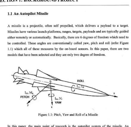
2.2

Optimal Control of MPC

uts Past inp and outp

Future inputs

uts

.

Model

Predicted outputs

-'"

Reference trajectory

+

Optimiser

Future error

s

Cost

[image:15.505.30.476.80.790.2]

function Constraints

(16)

The basic structure to implement MPC strategy shows in figure 2.1. There are two

important blocks as illustrates above, which are model and optimiser. Hence, it is true

that the essence of MPC as well as PFC is to optimise, over the manipulability inputs,

predicting of the process behaviour given [6]. A model is used to predict the future plant

outputs, based on past and current values and on the proposed optimal future control

actions. These actions are calculated by the optimizer taking into account the cost

function as well as the constraints.

2.3 Formulation of PFC Algorithm

2.3.1 Models

The model is the essential element of an MPC controller [ 6] and hence, also for

PFC controller. PFC can use many forms of model i.e.; internal model (IM),

including state space, transfer function, Finite Impulse Response (FIR), fuzzy

rules, and etc. The use of IM is important in PFC to capture the process dynamics

of the system and also continue to calculate the PFC control law later on.

2.3.2 State-space Model

Hence, for this section, the model will be developed in state-space form. The

discussion of PFC and other MPC algorithms in state-space form has several

advantages, including easy generalisation to multivariable systems, ease of

analysis of closed-loop properties, and online computation [6].

Given the general state space model, of the form:

! k+1

=

A!k

+

B?!.k ｾｫ＠ =C!k +D?!.k

Prediction with a strictly proper system (D

=

[O])

ACS6200: Predictive Functional Control (PFC) For Use in Autopilot Design

(2.1)

(17)

:!k+2

=

A:!k+i

+

ｂｾｫＫＱ＠

Y -Cx

- k+2 - -k+2

Substituting Equation 2.1 into 2.2;

:!k+3

=

A2 [A:!*

+

ｂｾｊＫ＠

ａｂｾｫＫｩ＠

+

ｂｾｫＫＲ＠

ｾｫＫＳ＠

=

C:!k+3

This process is simply an iteration of a one step ahead prediction, repeated

substitutions result in the prediction matrices, P and H.

An An-IB An-2B B

:!k+n

=

:!k

+

ｾｫ＠

+

ｾｫＫｉ＠

+ •• · +

ｾｫＫｮＭＱ＠

ｾｫＫｮ＠

=

c[An :!k

+

An-1

ｂｾＪ＠

+ An-1

ｂｾｫＫＱ＠

+ ... +

ｂｾｫＫｮＭＱ｝＠

State Prediction Equation

! k+l

! k+2

! k+J

! k+n

f..xx

B 0 0

AB B 0

A2B AB B

Hxx

Output Prediction Equation

.l::'. k+l .l::'. k+2 .l::'. k+J

}:'. k+n =

=

0 CB CAB H

... 0 ... 0 ... 0 ... 0

... B

0 0

CB

Y. k Y. k+l Y. k+2 Y. k+n-1 ｾ＠ k-1 0 0 0 0 CB Y. k

Y. k +l

Y. k +2

Y. k+n-1

ｾ＠ k-1

(2.2)

(2.3)

(2.4)

(18)

From Equation 2.4 and 2.5 above, it shows the model used is a linear one that

represent by;

ｾｫ＠

=

Pxx!k

+

HxlJ.k-1

ｾｫ＠ =P!_k +HlJ.k-1 (2.6)

where !le is the state model, ｾ＠ is the input model, »is the measured output model,

P= Hxx, P and Hare respectively, matrices or vectors of the right dimension.

Below, the algorithm for PFC is outlined as found in [5]. There is an element of

derivation here, however its inclusion is necessary as it helps to explain the main

concepts behind PFC. This intuitive approach is one of the key selling points.

2.3.3 Reference trajectory formulation

PFC formulates the reference trajectory by placing the desired closed-loop

dynamic into the reference trajectory. Given the actual set point is r, the loop set

point w is a first order lag [3].

(2.7)

where Yk is the most recent measured output and '¥ ( 0 < '¥ < 1 ) is scalar and a tuning parameter setting the desired closed-loop pole.

The predictive essence of control strategy is completely included in Equation 2. 7

above. Indeed, the aim is to track the set point trajectory following the reference

desired closed-loop behaviour.

2.3.4 The coincidence points

The control law is determined by using the d.o.f to enforce equality of the

predictions and the reference trajectory at a number of points, that is, by solving

the control moves such that:

(19)

Y k+n

=

W k+n, n

=

n1,n2, ... . (2.8)

These equalities are called coincidence points. Typically, there only have one or

two coincidence points. However, in this paper will only concentrate with one

coincidence points only.

2.3.5 Paramerisation of the d.o.f/future control trajectory

The PFC takes the trajectory as the sum of a step change, a ramp, a parabola, etc.

The precise components to be included are selected to match the expected

characteristics in the set point.

2.3.6 Computational of the control law:

At a single coincidence points, and using equation 2. 7 and 2.8, the control law is

determined by;

(2.9)

Hence, substituting Equation 2.6 with 2.9;

(2.10)

By assuming g k + ;

=

g "' the control law can be computed by rewriting the

Equation 2.10 and obtain;

I .

M. k

= -

H [ P ! k

+ (

rk - (rk - y,J IP 1 ) ]

M. k

= -

K ! k

+

fJ

Tk

I .

where; K

= -

H ( P - IP 1

Yk)

fJ

= -HI (I - IP;)

(20)

Thus, it can easily express as a fixed linear feedback law in the form of prediction

algorithm. Hence conventional a posterior stability and sensitivity analysis can be

applied in straightforward manner.

2.3. 7

Tuning Parameters of PFC

The tuning parameters of PFC are generally the coincidence horizon, e.g. n1

=

1,

2, . . . and the desired time constant, \f. The typical procedure with one coincidence point [3] would be as follows:

1. Choose the desired \f.

2. Do a search for n1

=

1, ... large and find the associated control law for each

n1.

3. Select the n1 which gives closed-loop dynamics closest to the chosen \f.

4. Simulate the proposed law. Otherwise, reselect \f and go to step 2.

Hence, the tuning reduces to a global search, but this requires only relatively

trivial computations and hence would be quite quick. With two coincidence

points, the global search would be more involved but should still be quick.

2.4 PFC for unstable Process

2.4.1 Introduction

PFC algorithm is defined in the previous sub-section is basically open-loop

process control applications. In the contrary, in industry applications, open-loop

unstable processes do also occur. Yet, these systems are difficult to control.

Hence, systematic control design tools are needed to handle complex instability

without a high on-line computational load. ADERSA have successfully applied

PFC on many unstable systems [3]. This section will discuss the theoretical tools

to pre-stabilise the unstable plants to implement the stabilizing linear PFC control

formulation.

(21)

2.4.2 Unstable Open-Loop Problems

PFC, as well as other MPC algorithms is weak with both non-minimum phase

problems and some unstable process [3], or called prediction mismatch. If the

process open-loop is unstable, PFC and also MPC are ill-posed because prediction

cannot match desired behaviour of the process, i.e. diverging. Therefore,

divergence open-loop prediction is the main cause of the prediction mismatch.

Hence, there is a must to stabilise the prediction. There are two ways of

pre-stabilise the predictions which are inserting a stabilising loop and another by

shaping the future inputs, algebraically so that the outputs are stable. However,

this section only focused on solving algebraically the unstable process as

discussed by [7] and [8].

2.4.3 Predictive Stabilisation

Removal of the prediction mismatch is essential for PFC to work. Hence, the

model needs to have prediction stabilisation. One method is by cancelling the

unstable modes and starts working with stable predictions. This means that PFC

control law process must be modified. Therefore, in solving this problems PFC

will lead to good closed-loop performance if the predictions used are a good

match to the consequent closed-loop behaviour.

The illustration below shows the state space method of predictions to cancel the

unstable modes [3]. Let a state-space matrix have some unstable eigenvalues.

Decompose the system into stable and unstable modes using eigenvalue

decomposition;

A

[ w.

W.J diag[A.

A.J

｛ｾｾ＠

(2.12)

where subscript s is used for stable and u for unstable. Clearly if a state lies solely

(22)

(2.13)

Given this, the predicted state evolution would follow

i i T

ｾ＠ k+ ilk

=

A ｾ＠ k

=

Ws As

Vs

ｾ＠ k (2.14)

then the mode 2 predictions are given by

!:!. k+ nc+ ;=O (2.15)

By assuming there is no disturbances or measurement noise, then continue with

predict by iterating the model (Equation 2.1 ). So we get

ｾ＠ k + 111c ］ａｾ＠ k

+

B!:!. k!k

ｾ＠ k + 211c = A ｾ＠ k + 111c

+

B!:!. k + 111c = A2 ｾ＠ k +AB !:!. k!k

+

B!:!. k+ 11k

A; A ;.1 B B

ｾ＠ k + ilk = ｾ＠ k

+

!:!. klk

+ ... +

!:!. k + i -1/k

which can be summarized as

,i; "

v.

ｾ＠

A; ,i; ,

+ [

A;.J B

+

A;.i B ... B ) [ _!:!.!:!. k!k k +llk

l

!:!. k + i -1/ k

M

or in common form

To ､ｲｩｶ･ｾＫ＠ k + ilk = 0, from equation 2.13, we know that

VuT X k+ ilk= 0,

Hence, by substituting equation 2.18 with 2.17 and 2.12, we get; ACS6200: Predictive Functional Control (PFC)

For Use in Autopilot Design

(2.16)

(2.17)

(2.18)

(23)

T .

Vu [A'-! k

+

M !! k ]

=

0,

. T

So as clearly for Wu Au' Vu

=

0. Therefore;

T i i T

Vu [A -! k

+

Ws As Vs !! k + i ]

=

0

The control law becomes,

!! k + ;

= - [

Ws A/

V/

r

1

V/

Ai -! k

+HP

.J! k

= -

K -! k

+

HP

where K

= [

Ws A/ Vs T

r

1 Vu T Ai and

p

could be choose freely.

2.4.4 Closed-Loop Paradigm (CLP) Concepts

(2.19)

(2.20)

As mentioned above, PFC will lead to good closed-loop performance if the

predictions used are a good match to the consequent closed-loop behaviour.

Hence, the closed-loop paradigm (CLP) is introduced here. CLP, which was

originally proposed as part of an algorithm stable generalised predictive control

(SGPC, [9]) will be implemented in the modified PFC after the pre-stabilised

prediction.

2.4.5 CLP Predictions

Based on the prediction on the PFC algorithm, the equations within the

pre-stabilised loop during prediction are;

-! k+ilk

=A-!

k+i-llk

+

B!! k +;;

!! k+i

=

Ｍｾ＠ k+ilk

+

c k+i;

By removing the dependent variable y_ k + ; one gets;

(24)

:! k+ilk = /A - BK);! k+i-Ilk

+

B H,k +1,·

H. k+i ］Ｍｾ＠ k+ilk +

c

k+i;

Hence, simulating these forward in time with <P = A - BK one gets;

State Prediction Equation

! k+J

=

<!> B 0 0 0

! k+2 <1>2 <!> B 0 0

! k+J <l>J ! k

+

<1>2B <!> B 0

0

! k+n <!>"

<P"-1

B <l>n-2 B <l>"-JB B

:! k+n

f.

cl He

Or in more common form

:!k+n = f. c1 ｾｫ＠

+

H cfk+n

The corresponding input predictions can be written as

Input Prediction Equation

Y. k+l

=

- K - K<l>

- K</>2

Y. k+2

=

Y. k+J

=

! k

+

Y. k+n

H. k+n

f.

c/u

Or in more common form B -KB - K<l>B

H_ k+n= f. c1u ｾｫ＠

+

H cufk+n

0

B

-KB

The state after nc steps will be denoted as

ACS6200: Predictive Functional Control (PFC) For Use in Autopilot Design

Heu

0 0 B

f. k

f k+n

0 0 0

0 B

f. k

f k+n

Predictive functional control (PFC) for use in autopilot design.

University

EXECUTIVE SUMMARY

Introduction/Background

Aims and Objectives

Achievements

Conclusion I Recommendations

ACKNOWLEDGEMENT

HYREIL ANUAR KASDIRIN

CONTENTS

SECTION 2: PREDICTIVE FUNCTIONAL CONTROL (PFC)

LIST OF FIGURES

LIST OF TABLES

SECTION 1: BACKGROUND PROJECT

1.2 Predictive Functional Control (PFC)

1.3 Thesis Scenario: PFC as a controller of Autopilot Missile

1.4 Aims and Objectives

1.5 Chapter Outline

SECTION 2: PREDICTIVE FUNCTIONAL CONTROL (PFC)

2.1 Predictive Control and MPC Algorithm

ADERSA. [1], [3]

Optimal Control of MPC

2.3 Formulation of PFC Algorithm

2.3.1 Models

2.3.2 State-space Model

ａｂｾｫＫｩ＠

ｾｫＫＳ＠

ｾｫＫｮ＠

ｾｫ＠

2.3.3 Reference trajectory formulation

2.3.4 The coincidence points

2.3.5 Paramerisation of the d.o.f/future control trajectory

2.4 PFC for unstable Process

2.4.1 Introduction

2.4.2 Unstable Open-Loop Problems

2.4.3 Predictive Stabilisation

W.J diag[A.

2.4.4 Closed-Loop Paradigm (CLP) Concepts

2.4.5 CLP Predictions