CONTROLLER SYNTHESIS FOR POLYNOMIAL DISCRETE-TIME SYSTEMS.

(1)

http://researchspace.auckland.ac.nz

ResearchSpace@Auckland

Copyright Statement

The digital copy of this thesis is protected by the Copyright Act 1994 (New Zealand).

This thesis may be consulted by you, provided you comply with the provisions of the Act and the following conditions of use:

x Any use you make of these documents or images must be for research or private study purposes only, and you may not make them available to any other person.

x Authors control the copyright of their thesis. You will recognise the author's right to be identified as the author of this thesis, and due acknowledgement will be made to the author where appropriate. x You will obtain the author's permission before publishing any

material from their thesis.

To request permissions please use the Feedback form on our webpage.

http://researchspace.auckland.ac.nz/feedback

General copyright and disclaimer

In addition to the above conditions, authors give their consent for the digital copy of their work to be used subject to the conditions specified on the Library Thesis Consent Form and Deposit Licence.

Note : Masters Theses

The digital copy of a masters thesis is as submitted for examination and contains no corrections. The print copy, usually available in the University Library, may contain corrections made by hand, which have been

(2)

CONTROLLER SYNTHESIS FOR

POLYNOMIAL DISCRETE-TIME

SYSTEMS

by

Mohd Shakir Bin Md Saat

A Thesis Submitted in Partial Fulfilment of the Requirements for the Degree of

Doctor of Philosophy

in the

DEPARTMENT OF ELECTRICAL AND COMPUTER ENGINEERING FACULTY OF ENGINEERING

THE UNIVERSITY OF AUCKLAND

(3)

The University of Auckland

Thesis Consent Form

This thesis may be consulted for the purpose of research or private study provided that due acknowledgment is made where appropriate and that the author’s permission is obtained before any material from the thesis is published.

I agree that the University of Auckland Library may make a copy of this thesis for supply to the collection of another prescribed library on request from that library; and

1. I agree that this thesis may be photocopied for supply to any person in accordance with the provisions of Section 56 of the Copyright Act 1994.

Or

2. This thesis may not be photocopied other than to supply a copy for the collection of another prescribed library..

(Strike out 1 or 2)

Signed:

Date:

(4)

Abstract

The polynomial discrete-time systems are the type of systems where the dynamics of the systems are described in polynomial forms. This system is classified as an important class of nonlinear systems due to the fact that many nonlinear systems can be modelled as, transformed into, or approximated by polynomial systems.

The focus of this thesis is to address the problem of controller design for polynomial discrete-time systems. The main reason for focusing on this area is because the controller design for such polynomial discrete-time systems is categorised as a difficult problem. This is due to the fact that the relation between the Lyapunov matrix and the con-troller matrix is not jointly convex when the parameter-dependent or state-dependent Lyapunov function is under consideration. Therefore the problem cannot possibly be solved via semidefinite programming (SDP). In light of the aforementioned problem, we establish novel methodologies of designing controllers for stabilising the systems both with and without H∞ performance and for the systems with and without uncertainty. Two types of uncertainty are considered in this research work; 1. Polytopic uncertainty, and 2. Norm-bounded uncertainty. A novel methodology for designing a filter for the polynomial discrete-time systems is also developed. We show that through our proposed methodologies, a less conservative design procedure can be rendered for the controller synthesis and filter design.

In particular, a so-called integrator method is proposed in this research work where an integrator is incorporated into the controller and filter structures. In doing so, the original systems can be transformed into augmented systems. Furthermore, the state-dependent Lyapunov function is selected in a way that its matrix is state-dependent only upon the original system state. Through this selection, a convex solution to the con-troller design and the filter design can be obtained efficiently. However, the price we pay for incorporating the integrator into the controller and filter structures is a large computational cost, which prevents us from using this method in general. To reduce the computational requirements for our design methodologies a number of simpler classes of polynomial systems are considered.

(5)

iii ensures that the ratio of the regulated output energy and the disturbance energy is less than a prescribed performance level. The filter design is tackled next and followed by the output feedback control problem. In the output feedback control, the problem of system uncertainties and disturbances are addressed.

The existence of such controllers and a filter are given in terms of the solvability of polynomial matrix inequalities (PMIs). The problem is then formulated as sum of squares (SOS) constraints, therefore it can be solved by any SOS solvers. In this research work, SOSTOOLS is used as a SOS solver.

(6)

Acknowledgements

In the Name of Allah, the Most Merciful, the Bestower of Mercy. All praises are due to Allah, and may Allah exalt the status of the Messenger of Allah and that of his family and his companions, and may He grant them peace. Alhamdulillah, due to His guidance and will, this thesis finally managed to be completed successfully.

First and foremost, I would like to take this opportunity to express my heartfelt appre-ciation to my supervisor, Prof. Sing Kiong Nguang, for his enthusiasm, vision, wisdom and guidance throughout this research journey at the University of Auckland. There is no doubt that he is an outstanding and prominent researcher to have as a great role model for a Ph.D student. Throughout my Ph.D journey, he has given his full support and conveyed extensive knowledge that significantly led to the successful completion of this thesis. I am very sure that without the help from Prof. Nguang, this work could not have been accomplished. Furthermore, his many refinements to conference papers, journal articles and this thesis have been much appreciated. For this, I owe him my sincere gratitude. I hope that this relationship continues and I look forward to collabo-rating with him in the near future. Thank you Allah that I was destined to be a Prof. Nguang’s student.

I would also like to acknowledge my co-supervisor Dr. Nitish Patel and all the advisory committee members, for their insightful commentary and precious time serving on my committee. My special thanks go to Dr Akshya Swain for his constructive advice and comments, especially in the control group meeting. Indeed, his advice has helped me greatly in refining my work. Not to forget my colleagues in the control research group for their kind help and support throughout the completion of this thesis.

Here, acknowledgment also goes to the support staff at the Electrical and Computer Engineering Department. Throughout the years they have been very helpful. Thanks to Peter Wigan and Edmond Lo for their support in providing me with such a great computer facility. Every time I needed help, they were always there to help me out. Thank you both.

This thesis has been financially supported by The Ministry of Higher Education Malaysia (MoHe), The University of Technical Malaysia Malacca (UTeM) and The University of Auckland PreSS Account.

My deepest appreciation goes to my lovely father, Md Saat Bin Kamis, my lovely mother, Yah Binti Eyat, and my beloved parents-in-law, Ibrahim Che Mat and Azizah Ahmad for their ’Dua’, love, motivation, support, and encouragement. I pray to Allah to place all of you into ’Jannah’. I love you all very much. ’Abi’, today your dream is finally

(7)

v fulfilled, the dream to see one of your children achieve great success in education. Do you know why I have so much motivation in my study? It is all because of you. I want to see the tears of happiness in your eyes. I want to see you be the happiest person in this world. I want to prove to everyone that slandered you before that they are totally wrong. You are not that kind of person. I’m glad to have you as my father. I love you so much with a love that is never ending. Not to forget to my brothers and sisters for their help and support that significantly led to the success of this Ph.D. Thank you very much for everything and I cannot wait to gather together and talk with you all.

(8)

List of Figures

1.1 Schematic diagram of a computer-controlled system. . . 3

1.2 Diagram depicting how SOS programs (SOSPs) are solved using SOS-TOOLS. . . 18

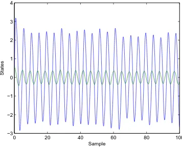
2.1 The trajectory for the open-loop uncertain Hennon Map with a=1.4 and b=0.3. . . 33

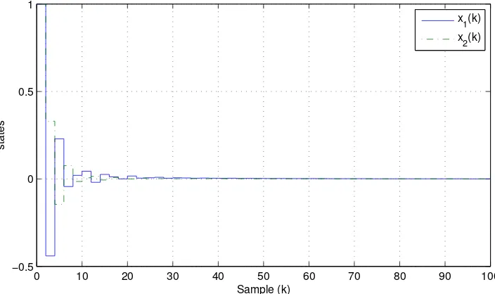
2.2 Response of plant states for nonlinear feedback controller. . . 34

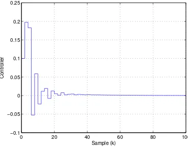
2.3 Controller responses for nonlinear feedback control. . . 34

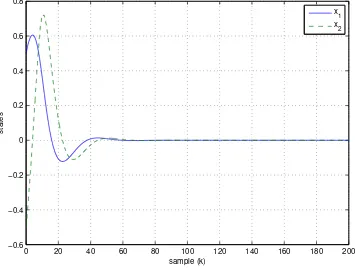
2.4 Response of the plant states for the uncertain system. . . 36

2.5 Controller responses for the uncertain system. . . 37

3.1 System states for uncertain discrete-time systems. . . 46

3.2 Controller Responses. . . 46

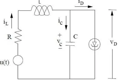
4.1 A Tunnel diode circuit.. . . 56

4.2 Open loop responses for a Tunnel diode circuit. . . 58

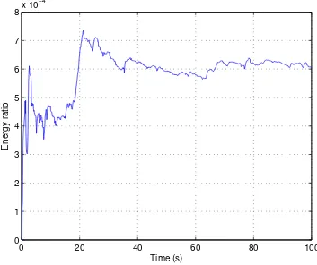
4.3 Ratio of the regulated output energy to the disturbance input noise energy without uncertainty. . . 59

4.4 Energy ratio of the regulated output and the disturbance input noise with polytopic uncertainties. . . 60

5.1 energy ratio:PPzTz ωT_ω ≤γ2.. . . 69

6.1 Trajectory of the ˆx1−x1. . . 77

6.2 Trajectory of the ˆx2−x2. . . 78

7.1 Tunnel diode circuit. . . 98

7.2 Ratio of the regulated output energy to the disturbance input noise energy of a tunnel diode circuit. . . 101

7.3 Ratio of the regulated output energy to the disturbance input noise energy of a tunnel diode circuit with polytopic uncertainty. . . 102

8.1 Ratio of the regulated output energy to the disturbance input noise energy of a tunnel diode circuit. . . 113

(12)

List of Tables

1.1 Example of Polynomial Systems. . . 18

(13)

Abbreviations

A-D Analogue to Digital BMI Bilinear Matrix Inequality D-A Digital to Analogue

HJI Hamilton Jacobi Inequality LMI Linear Matrix Inequality LPV Linear parameter varying NP Nondeterministic Polynomial PD Positive Definite

PMI Polynomial Matrix Inequality PSD Positive Semidefinite

SDP Semidefinite Programming SOS Sum of Squares

SOSP Sum of Squares Program TS Takagi Sugeno

ZOH Zero Order Hold

(14)

Notations

The notation used in this thesis is quite standard. Rn and Rn×m

denote respectively the set ofn_×1 vectors, and the set of all n_×mmatrices. The superscript T denotes the transpose and_∗ is used to represent the transposed symmetric entries in the matrix inequalities. In addition I represents the identity matrix and L2[0,∞] is the

space of square summable vector sequence over [0,_∞]. The_k._k_[0_,∞_] denotes theL2[0,∞]

norm over [0,_∞] defined as _kf(x)_k2_[0_,∞_]=

P∞

0 kf(x)k

2_{. The positive definiteness of the}

matrixQ(x(k)) is denoted byQ(x(k))>0 andQ(x(k))<0 denotes the negative definiteness of theQ(x(k)). Sometimes, for the notation simplicity we write P(x+)

to denote P(x(k+ 1)).

(15)

To my parents, parents-in-law, family, lovely wife and kids. . .

(16)

Chapter 1

Introduction

The purpose of this chapter is generally to emphasise the theory of nonlinear discrete-time systems, and the theory of polynomial discrete-discrete-time systems in particular. We begin this chapter by describing the concept of nonlinear systems and nonlinear discrete-time systems. Then, available methods for stabilizing nonlinear discrete-time is provided. Furthermore, the fundamental concept of polynomial systems is given and followed by the overview of the existing literature dealing with the controller synthesis for polyno-mial systems. As the sum of squares method is used for solving the controller and filter design problems, hence the description of sum of squares decomposition method is also highlighted in this chapter. Next, the motivation of delivering this research work is pre-sented and followed by the contribution of this research work. This chapter is concluded with the outline of the thesis, highlighting the summary of each chapter.

1.1

Nonlinear Systems

Nonlinear systems play a vital role in the control systems engineering point of view. This is due to the fact that in practice all plants are nonlinear in nature. This is the main reason for considering the nonlinear systems in our work. In mathematics, a nonlinear system is one that does not satisfy the superposition principle, or one whose output is not directly proportional to its input. The best example to explain nonlinearity is obviously a saturation. This condition exists because it is impossible to deliver an infinite amount of energy to any real-world system.

(17)

Chapter 1. Introduction 2 In general, the state equations and output equations for the nonlinear systems may be written as follows:

˙

x(t) =f[x(t), u(t)]

y(t) =g[x(t), u(t)] (1.1)

The Lorenz chaotic system is one of the example of nonlinear systems which is described as below:

˙

x1(t) =−10x1(t) + 10x2(t) +u(t)

˙

x2(t) =28x1(t)−x2(t) +x1(t)x3(t)

˙

x3(t) =x1(t)x2(t)−

8

3x3(t) (1.2) Notice that the terms x1(t)x3(t) and x1(t)x2(t) exist in the equation (1.2), hence the

system (1.2) is nonlinear in nature . In the sequel, the nonlinear discrete-time systems is introduced because it will be considered in this research work.

1.2

Nonlinear Discrete-Time Systems

Nowadays we can see that almost all controllers are implemented using computers. These kinds of controller are known as digital controllers. Basically, the use of digital controllers has rapidly increased since the first idea of using digital computers as one of the com-ponents in control systems emerged somewhere in 1950. The detailed history of this development can be found in [1]. The main reason for this development is due to the advances in hardware, hence it provides the control engineer with more powerful, reli-able, faster and above all cheaper computers that could be implemented as process con-trollers. The another significant factor that drives the increase in development of digital controllers is the advantage of working with digital signals rather than continuous-time signals [2]. The aforementioned factors generally motivate us to deliver the research in the framework of discrete-time systems rather than continuous-time systems.

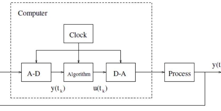
Generally, a closed loop system of computer controlled systems can be illustrated as Figure 1.1. From Figure 1.1 the output of the processy(t) is a continuous-time signal. The measurements of the output signal are fed into an analog-to-digital (A-D) converter, where the continuous-time signal is converted into a digital signal - a sequence of mea-surements at sampling times tk. At this point, if a digital measurement device is used,

(18)

Chapter 1. Introduction 3 taken at sampling times only. The computer interprets the converted output signals,

y(tk) as a sequence of numbers, and this sequence is then used by the control algorithm

to compute a sequence of digital control signals, u(tk). Notice that the process input is

in continuous-time, hence a digital-to-analog (D-A) is used to transform the signals into a continuous-time signal. It is important to highlight here that between the sampling in-stants the system is in open loop mode. The system is synchronised by a real time clock in the computer. Consequently, the inter-sample behaviour is very often an issue and should not be disregarded. However, in many applications it is sufficient to describe the dynamic behaviour of the system at the sampling instants. At this stage, the interested signals are only at discrete-time, and this system is classified as a discrete-time system [1,3]. We can now simply justify that if the dynamic of the process is in linear forms, then such a system is called a linear discrete-time system. Meanwhile if the behaviour of the process is nonlinear, then it is known as a nonlinear discrete-time system.

Figure 1.1: _{Schematic diagram of a computer-controlled system.}

1.2.1 Discretization

With the fact that systems in this world are naturally in continuous-time, discretization shall be performed so that an approximated discrete-time system can be obtained. Listed below are the available methods in the discretization framework:

• Euler’s Forward differentiation method and Euler’s Backward

differ-entiation method: The methods are based on the approximations of the time

(19)

Chapter 1. Introduction 4 but it is simpler to use. Particularly, with nonlinear models the backward differ-entiation may give problems since it results in an impact equation for the output variable. In contrast, the forward differentiation method always gives an explicit equation to the solution.

• Zero Order Hold (ZOH) method: Using this method, it is assumed that the

system has a zero order hold element on the input element of the systems. This is the case when the physical system is controlled by a computer via digital-to-analogue (D-A) converter. ZOH means that the physical input signal to the system is held fixed between the discrete points. Unfortunately, this method is relatively complicated to apply, and in practice the computer tool i.e MATLAB or LabVIEW can perform the job.

• Tustin’s method: The discretization method is based on an integral

approxima-tion where the integral is interpreted as the area between the integrand and the time axis, and this area is approximated with trapezoids. It should be noted here that in Euler’s method this area is approximated by a rectangle.

• Tustin’s method with frequency prewarping, or Bilinear transformation:

This method follows Tustin’s method but with a modification so that the frequency response of an original continuous-time system and the resulting discrete-time sys-tems have exactly the same frequency response at one or more specified frequencies. It should be mentioned here that discretization methods are not the main focus of this thesis. The discretization is only applied in the simulation examples as to convert the continuous-time systems into discrete-time systems. To perform such a discretization, in this research work, the Euler’s method is used due to its simplicity.

1.2.2 Brief Overview on The Literature of Nonlinear Discrete-time Systems

(20)

Chapter 1. Introduction 5 major drawback of the feedback linearisation approach. With this knowledge, a signifi-cant amount of works can be found in the literature which attempts to provide a more general and a less conservative result than the linearised approach. One of the popular approaches is obviously backstepping control technique [5]. This approach is actually a combination of two popular theories, Lyapunov stability theory and the geometric method. By exploring the recursive design procedure, the time-varying uncertainties and parameter uncertainties can be incorporated in the problem formulation. However, it is difficult to find a general class of Lyapunov functions that could ensure the stability of such systems. This is the main disadvantage of backstepping control techniques, and obviously this drawback is common to all approaches that uses a constructive procedure in developing Lyapunov candidates [6].

Besides the existence of feedback linearisation and backstepping control techniques for stabilising nonlinear systems, there is one more popular method available that is widely used in control systems engineering, this method is called gain-scheduling [7]. The primary advantage of gain-scheduling for nonlinear control design is that it is usually possible to meet performance objectives over a wide range of operating conditions while still taking advantage of the wealth of tools and designers experience from linear con-troller synthesis. From this gain-sceduling approach, a more systematic control design technique is developed in the framework of linear parameter varying (LPV) systems with guaranteed stability and performance properties [8–10]. However it is important to highlight here that the stability and performance properties of the LPV systems only hold locally and it is well known that the application of LPV control techniques always requires one to convert the nonlinear systems into their quasi-LPV forms. These are usu-ally the main sources of conservatism of this gain-scheduling method. Another popular approach in this area is based on the Fuzzy Takagi-Sugeno approach. It is well known that Takagi-Sugeno Fuzzy models can be used to approximate nonlinear systems [11–13]. However, in the TS fuzzy model, the premises variables are assumed to be bounded. In general, the premise variables are related to the state variables which implies that the state variables have to be bounded. This is one of major drawbacks of the TS fuzzy model approach.

(21)

Chapter 1. Introduction 6 the scope, where only the polynomial discrete-time systems will be considered. The reason for selecting the polynomial system will be given in the following text.

1.3

Polynomial Systems

It is well known that a wide class of nonlinear systems can be exactly represented by polynomial systems: i. e Lorenz chaotic systems. Moreover, the polynomial system has an ability to approach any analytical of nonlinear systems. These advantages explain why the polynomial system constitutes an important class of nonlinear systems and has attracted considerable attention from control researchers to involve themselves in this area, especially on the stability analysis and controller synthesis of polynomial systems [14].

The polynomial systems are the systems where the dynamic of the system is given in terms of polynomial functions or polynomial matrices. The general polynomial systems can be described as follows:

˙

x(t) =f(x(t), u(t))

y(t) =g(x(t)) (1.3) where f(x(t), u(t)) and g(x(t)) are in polynomials forms, and x(t), u(t) and y(t) are respectively the states, input and the measured output.

Meanwhile, in discrete-time, the (1.3) can be written as follows:

x(k+ 1) =f(x(k), u(k))

y(k) =g(x(k)) (1.4) where f(x(k), u(k)) andg(x(k)) are in polynomials forms, and x(k), u(k) and y(k) are respectively the states, input and the measured output of the system at sampling time,

k. More precisely, the class of polynomial systems that is under consideration in this research work is described in terms of a state-dependent linear-like form as follows:

˙

x(t) =A(x(t))x(t) +B(x(t))u(t)

(22)

Chapter 1. Introduction 7 In our work, the polynomial discrete-time system is described as follows:

x(k+ 1) =A(x(k))x(k) +B(x(k))u(k)

y(k) =C(x(k))x(k) (1.6) where, x(k) _∈ Rn _{is the state vectors,} _u₍_k₎ _∈ _Rm _{is the input and} _y₍_k_{) is the}

mea-sured output. A(x(k)), B(x(k)) and C(x(k)) are polynomial matrices of appropriate dimensions.

Given below are the examples of the polynomial systems:

Example 1: The Lorenz Chaotic Systems

˙

x1(t) =−10x1(t) + 10x2(t) +u(t)

˙

x2(t) =28x1(t)−x2(t) +x1(t)x3(t)

˙

x3(t) =x1(t)x2(t)−

8

3x3(t) (1.7)

Example 2: A Tunnel Diode Circuit

Cx˙1(t) =−0.002x1(t)−0.01x31(t) +x2(t)

Lx˙2(t) =−x1−Rx2(t) +u(t) (1.8)

whereC is a capacitor value, Lis inductance andR is a resistor.

One can see here that the systems given in (1.7)-(1.8) are actually nonlinear systems. These two examples illustrate the validity of the statement that we claimed earlier that many nonlinear systems can be represented by polynomial forms. It is also important to stress here that in this research we are not focusing on the method of discretizing the nonlinear systems to yield their discrete-time version. But, our main focus is to perform the controller synthesis for polynomial discrete-time systems.

1.3.1 Recent Work on Polynomial Systems

(23)

Chapter 1. Introduction 8 it is actually complementary to the LMIs approach. A detailed description regarding the SOS decomposition method will be provided later in this chapter.

The controller synthesis or stabilisation problem is one of the important areas in the research of polynomial systems. Therefore, considerable attention has been devoted to this framework; for instances, see [16–21,24–27]. In this present work, numerous tech-niques have been proposed to address the controller design problem for the polynomial systems. The brief of the proposed techniques is described below:

1. Dissipation inequalities and SOS: Dissipativity theory is known to be one

of the most successful methods of analysing and synthesising the nonlinear con-trol systems [15]. Mathematically speaking, this method is known as dissipation inequalities and has major advantages on the analysis and design of nonlinear sys-tems. This might be due to the fact that the investigation of a possibly large number of differential equations, given by the control system description, is re-duced to a small number of algebraic inequalities. Hence, the complexity of the analysis and design task is usually essentially reduced. In [16], the dissipation inequalities together with the SOS programming have been utilised to stabilise such polynomial systems. In particular, the authors represent their systems to be of descriptor systems or differential-algebraic systems where the functions are described by polynomial functions. They have managed to obtain the affine dissi-pation inequalities by the proposed method, hence the inequalities can be solved computationally via SOS programming. However, the process of achieving the affine dissipation inequalities varies for different types of problem. This means that the proposed method might not work for other problems.

2. Kronecker products and LMIs: The stabilisation of polynomial systems using

Kronecker products method can be found in [17–19]. In the present papers, the polynomial systems have been simplified using the Kronecker product and power of vectors and matrices. Moreover, a new stability criterion for polynomial sys-tems has been developed. A sufficient condition for the existence of the proposed controller is given in terms of the linear matrix inequalities (LMIs). The pro-posed controller can be applied to high order polynomial systems. This is the main advantage of this method. The strength of this approach comes from the solid theoretical results on the Kronecker products and the power of vectors and matrices.

3. Semi-tensor products: The semi-tensor product of matrices is a generalisation

(24)

Chapter 1. Introduction 9 A brief survey for the related materials can be found in [20]. The advantage of this method is the general polynomial systems can be considered without any homoge-nous assumption. In [20], a method to stabilise the polynomial systems has been developed. The present paper first proposes a sufficient condition for a polynomial to be positive definite. Then, the formula for the time derivation of a candidate polynomial Lyapunov function with respect to a polynomial systems is provided. Through the sufficient condition, the candidate of the Lyapunov function can be checked for the positive definiteness, and its derivative to be negative definite. The sufficient condition is given by a set of linear algebraic inequalities. However, us-ing this method, to choose a suitable candidate for the Lyapunov function is hard because there is no unique way to choose that Lyapunov function. The incorrect selection of the Lyapunov candidate leads the linear algebraic inequalities to have no solution. This is the main challenge of applying this method in the framework of controller synthesis for polynomial systems.

4. Theory of moments and SOS:Interesting work on the polynomial stabilisation

that utilises a theory of moments can be found in [21]. It has been known for a long time that the theory of moments is strongly related to-and in fact, in duality with the theory of nonnegative polynomials and Hilbert’s 17th problem on the representation of nonnegative polynomials [22]. In the light of this duality rela-tionship, the author in [21] study the problem of polynomial systems stabilisation. They managed to show that the global solution to the problem can be obtained in a less conservative way than the available approaches, and the solution can be solved easily by SDP [23]. However, in order to achieve a convex solution to the controller synthesis problem, the Hermite stability criterion is used rather than the Lyapunov stability theorem. In doing so, the controller matrix can be decoupled from the Lyapunov matrix and the solvability conditions of the proposed controller are developed through a hierarchy of convex LMI relaxations. As stated by the authors, this methodology suffers from the large number of constraints in a PMI which consequently leads to the need for reliable numerical software to handle the problem.

5. Fuzzy method and SOS:T-S fuzzy model is well known to be good at

(25)

Chapter 1. Introduction 10 the other hand, [25] proposed an improved sum-of-squares (SOS)-based stability analysis result for the polynomial fuzzy-model based control system, formed by a polynomial fuzzy model and a polynomial fuzzy controller connected in a closed loop. Two cases, namely perfect and imperfect premise matching, are considered. Under the perfect premise matching, the polynomial fuzzy model and polynomial fuzzy controller share the same premise membership functions. While different sets of membership functions are employed, it falls into the case of imperfect premise matching. Based on the Lyapunov stability theory, improved SOS-based stability conditions are derived to determine the system stability and facilitate the con-troller synthesis. approach. The application of polynomial fuzzy T-S approach to the two-link robot arm can be found in [26]. Meanwhile, for static output control, the result can be found in [27]. However, in the TS fuzzy model, the premises variables are assumed to be bounded. In general, the premise variables are related to the state variables which implies that the state variables have to be bounded. This is one of the major drawbacks of the TS fuzzy model approach.

6. Lyapunov method and SOS:This is the common method that is widely applied

in the literature for stabilising polynomial systems. This method is used in this research work and therefore the complete literature of this framework is provided in the following text.

1.3.1.1 On Literature Of Controller Synthesis For Polynomial Systems: The

Lyapunov Method and SOS Decomposition Approach

It is well known that Lyapunov’s stability theory [28] is one of the most fundamental pillars in control theory. Although this method was introduced more than hundred years ago, it remains popular among control researchers. This success is owed to its simplicity, generality, and usefulness. The Lyapunov’s stability is a method that was developed for analysis purposes. However, it has become of equal importance for control designs over the last decades [6]. The Lyapunov’s stability theory can be generalised as follows: Let us consider the problem of solving the stability for an equilibrium of a dynamical systems, ˙x = f(x) using the Lyapunov function method. It is clear that to find a stability using the Lyapunov method, we need to find a positive definite function of Lyapunuv function, V(x) defined in some region of the state space containing the equilibrium point whose derivative ˙V = dv_dxf(x) is negative semidefinite along the system trajectories. Take the linear case for instance, ˙x = Ax, these conditions amount to finding a positive definite matrix P, such thatATP +P Ais negative definite [29]; then the associated Lyapunov function is given by V(x) = xT_{P x}_{. Meanwhile for}

(26)

Chapter 1. Introduction 11 the positive definite function of Lyapunov function,V(x) defined in some region of the state space containing the equilibrium point whose difference of the Lyapunov function, ∆V = xT(k+ 1)P x(k + 1)₋xT(k)P x(k) is negative semidefinite along the system trajectories. The associated Lyapunov function is given by V(x) =xTP x.

Since the SOS decomposition technique introduced about 10 years ago [30], the system analysis for polynomial systems can be performed more efficiently because it helps to answer many difficult questions on system analysis that were hard to answer before. The popularity of this method grew quickly among the community of control researchers because the algorithmic analysis of nonlinear systems can be delivered using a most popular method, which is the Lyapunov method (as discussed earlier). Generally, the most interesting and important point that was never seen until recently is that both the amount of proving the certificates of the Lyapunov function V(x) and ₋V˙(x) can be reduced to the SOS [30]. Notice that for small systems, the construction of the Lyapunov function can be done manually. The difficulty of this construction is solely dependent upon the analytical skills of the researcher. However, when the vector field of the systems, f(x) and the Lyapunov function candidate V(x) are in polynomial forms, then the Lyapunov conditions are essentially is polynomial non-negativity conditions which can be NP-hard to test [45]. This is probably due to the lack of algorithmic constructions of Lyapunuv functions. However, if these nonnegativity conditions are replaced by the SOS conditions, then not only testing the Lyapunov function conditions -but also constructing the Lyapunov function can be done effectively using SDP [30]. This is the main advantage of using the SOS decomposition approach because the solution is indeed tractable. We will further describe the detail of the SOS decomposition method later.

(27)

Chapter 1. Introduction 12 The more recent and less conservative results can be found in [33]. In this paper, the effect of the nonlinear terms that exist in the problem formulation is described as an index, so that the control problem can be transformed into a tractable solution and can be possibly solved via SDP [23]. The optimisation approach is proposed to find a zero optimum of this index and solved using SOS programming effectively. However, to render a convex solution, the authors follow the same assumption as made in [32]. An improved version of the aforementioned approach can be found in [34] where an addi-tional matrix variable is introduced to decouple the Lyapunov matrix from the system matrices. Therefore, the controller design can be performed in a more relaxed way and the proposed methodology can be extended to the robust control problem of polynomial systems. However, to obtain a convex solution, the non convex term is bounded by an upper bound. Therefore, the stability can only be guaranteed within the bound region. Sometimes it is difficult to synthesise a controller that works globally. Besides, in a restricted region, local controllers often provide a better solution than global controllers. Some developments of this field can be found in [35, 36]. In [35], a rational Lyapunov functions of states was used to synthesise the polynomial systems. The variation of states is bounded, and the domain of attraction was embedded in the specified region by the nonlinear vector. With this, the state feedback controller is established and formulated as a set of polynomial matrix inequalities and solved using any SOS programming. The coupling between system matrices and the Lyapunov matrix causes the results to be quite conservative in general. Hence, [36] relaxes this issue by introducing a slack variable matrix. In doing so, the Lyapunov matrix is decoupled from the system matrices. Now, the parameterisation of the resulting controllers is independent of the Lyapunov-matrix variables. This allows them to extend their result to construct robust controller for uncertain polynomial systems using state-dependent Lyapunov functions.

(28)

Chapter 1. Introduction 13 show that their approach is less conservative than the available approaches and provides more general results in this field. But the main disadvantage of this approach is the selection of the initial polynomial function, ǫ(x), which is hard to choose because it is unknown.

The above-mentioned results are dedicated to solving the polynomial continuous-time systems. In regard to the polynomial discrete-time systems, there are only few results available which utilises the SOS decomposition method in their approach. The first result is proposed in [41], where the authors employ a state-dependent polynomial Lyapunov function as their Lyapunov candidates. Then, some transformations are required to represent the system with the introduction of new matrices (in polynomial). Furthermore YALMIP and PENOPT for PENBMI [42, 43] have been utilised to solve the problem. However, the main drawback of this approach is that the selected new matrices are not unique and hence difficult to choose. The most recent result was addressed by [44], where the nonconvex term is bounded by an upper bound value, then optimisation is carried out to find a zero optimum for the nonlinear term. Here, the problem was formulated as SOS and could be solved by using any SOS solvers. By bounding the nonconvex terms, the controller that resulted from this method can only guarantee the closed-loop stability within bounds. This is similar to the method proposed in [33,34]. Therefore, they share the same weaknesses as encountered in [33,34].

1.3.2 Sum of Squares(SOS) Decomposition

A brief overview of a SOS decomposition method is given in this section. A more detail description of the SOS decomposition method can be referred in [30].

Generally, proving a nonnegativity of multivariable functions is considered as one of the important aspects in control systems engineering. This problem is similar to the problem of proving the nonnegativity of a Lyapunov function. If the nonlinear system is concerned, then it is hard to prove the nonnegativity of such systems. Basically, the problem is to prove that

F(x1, ..., xn)≥0 x1, . . . , xn∈ ℜ (1.9)

A great amount of research has been devoted to proving (1.9). However, up to now there is no unique solution to the problem in (1.9).

(29)

Chapter 1. Introduction 14 It has been shown in [30], that considering the case of polynomial functions is a good compromise for this issue.

Definition 1.1. [30]: A form is a polynomial where all the monomials have the same

degree d := P

iαi. In this case, the polynomial is homogenous of degree d, since it

satisfiesf(λx1, . . . , λxn) =λdf(x1, . . . , xn).

It should be highlighted here that the general problem of testing global positivity of a polynomial function is NP-hard problem (when the degree is at least four) [45]. There-fore, a problem with a large number of variables will have unacceptable behaviour for any method that is guaranteed to obtain the right answer in every possible instance. This is actually the main drawback of theoretically powerful methodologies such as the quantifier elimination approach [46,47].

The question now is: are there any conditions to guarantee the global positivity of a tested polynomial time functions? This question underlines the existence of SOS decom-position approach [30] as one condition to guarantee the global positivity of polynomial functions.

It is obvious that a necessary condition to satisfy a polynomialF(x) in (1.9) is that the degree of the polynomial in the homogeneous case must be even. Hence, a simple suffi-cient for a real-valued functionF(x) to be positive everywhere is given by the existence of a SOS decomposition:

F(x) =X

i

fi2(x) (1.10)

It can been seen that ifF(x) can be written as (1.10), the nonnegativity ofF(x) can be guaranteed. It is stated in [30] that for the problem to make sense, some restriction on the class of functions fi has to be imposed again. Otherwise, we need to always define f1 to be the square root ofF, but, this results the condition both useless and trivial.

It has been shown in [30] that F(x) is a SOS polynomial if and only if there exists a positive definite matrix Qsuch that

F(x) =zTQz (1.11) wherez(x) is the vector of all monomials of degree less than or equal to the half degree ofF(x). This is the idea given in [51] and it can be shown to be conservative in general. The main reason is that since the variables zi are not independent, the representation

(30)

Chapter 1. Introduction 15 the zi variables among themselves, it is easily shown that there is a linear subspace of

matrices Q that satisfy (1.11). If the intersection of this subspace with the positive semidefinite matrix cone is nonempty for the original function, F is guaranteed to be SOS and therefore psd. So, ifF can indeed be written as the SOS of polynomials, then expanding in monomials will provide the representation (1.11). The following example explains this concept.

Example 1 [30] : Consider the quartic form in two variables described below, and define

z1; =x12.z2 :=x22, z3:=x1x2:

F(x1, x2) = 2x14+ 2x13x2−x12x22+ 5x24

=

   

x12

x22

x1x2

    T    

2 0 1 0 5 0 1 0 ₋1

       

x12

x22

x1x2

    =    

x12

x22

x1x2

    T    

2 ₋λ 1

−λ 5 0

1 0 ₋1 + 2λ

       

x12

x22

x1x2

   

(1.12)

Take for instanceλ= 3. In this case,

Q=LTL, L= √1 2

"

2 ₋3 1 0 1 3

#

(1.13) Therefore we have the sum of squares decomposition:

F(x1, x2) =

1 2((2x1

2

−3x22+x1x2)2+ (x22+ 3x1x2)2) (1.14)

Parrilo [30] also observed that the existence of (1.11) can be cast as a semidefinite programming [23]. This is the most important property that distinguishes its from other approaches. This feature is proved to be critical in the application to many control related problem. How does it works? Basically by expanding the zTQz and equating the coefficient of the resulting monomials to the ones in F(x), we obtain a set of affine relations in the elements of Q. We know that, for F(x) being a SOS is equivalent to

Q_≥0, the problem of findingQthen which provesF(x) is an SOS can certainly be cast as a semidefinite program.

(31)

Chapter 1. Introduction 16 significance results in suggesting that the relaxation is not too conservative in general. It must be noted here that as the degree of F(x) is increased or its variables number is increased, then the computational complexity for testing whetherF(x) is a SOS is sig-nificantly increased. Nonetheless, the complexity overload is still a polynomial function of these parameters.

In general, the conversion from SOS decomposition to the semidefinite programming can be manually done for small size instance or tailored for specific problem classes. However, this such conversion is cumbersome in general. Thus the software is absolutely necessary to aid in converting them. Specifically, the relaxation uses Gram Matrix methods to efficiently transform the NP-hard problem, into linear matrix inequalities (LMIs) [29]. These can in turn be solved in polynomial time with semidefinite program-ming (SDP) [23,29]. To date, there exist several freely available toolboxes to formulate these problems in Matlab, for example SOSTOOLS [53], YALMIP [54], CVX [55], and GLoptiPoly [56]. Whereas SOSTOOLS is specifically designed to address polynomial nonnegativity problems, the latter toolboxes have further functionality, such as modules to solve the dual of the SOS problem, the moment problem.

In this work we use SOSTOOLS to perform this conversion for our problem formulation. Hence we will describe the working principles of this software in the following section. Basically the polynomial case is a well-analysed problem, first studied by David Hilbert more than century ago [48]. He raised a very popular and important questions in his famous list of twenty-three unsolved problem which was presented at the International Congress of Mathematicians in Paris, 1900, dealing with the representation of a definite form as a SOS. Hilbert also noted that not every positive semidefinite (psd) polynomial (or form) is sos. However, [49] has proved that the numerical examples seem to indicate that the gap between the SOS and nonnegativity polynomial is small. A complete characterisation has been outlined by Hilbert in explaining when these two classes are equivalent. There are three cases which the equality holds: 1. The case with two variables (n= 2), 2. The familiar case of quadratic form (i.e, m = 2), 3. A surprising case, where P3,4 =P3,4, refer [50] for detailed explanations.

Before ending this section, the following lemma is presented and it is useful for our main results later.

Lemma 1.2. [32] Let F(x) be an N_×N symmetric polynomial matrix of degree 2d in

x _∈Rn_{. Furthermore, let} _Z₍_x₎ _{be a column vector whose entries are all monomials in} x with a degree no greater than d, and consider the following conditions:

(32)

Chapter 1. Introduction 17

2. vTF(x)v is a SOS, wherev_∈RN

3. There exists a positive semidefinite matrix Q such that

vT_F₍_x₎_v_{= (}_v_⊗_Z₍_x₎₎T _Q₍_v

⊗Z(x)), with _⊗denoting the Kronecker product It is clear that F(x) being a SOS implies F(x) _≥ 0, but the converse is generally not true. Furthermore, statement (2) and statement (3) are equivalent.

1.3.2.1 SOSTOOLS

SOSTOOLS is a free, third-party MATLAB toolbox specially designed to handle and solve the SOS programs. The techniques behind it are based on the SOS decomposition for multivariate polynomials, which can be efficiently computed using semidefinite pro-gramming frameworks. The availability of SOSTOOLS gives a great advantage to the researchers that involved in SOS polynomial frameworks. Moreover, the SOSTOOLS gives a new direction for solving many hard problems such as global, constrained, and boolean optimisation due to the fact that these technique provide a convex relaxations approach.

The working principles of SOSTOOLS is shown in figure 1. Basically, the SOSTOOLS will automatically convert the SOS program (SOSP) into semidefinite programs (SDPs). Then, it calls the SDP solver, and converts the SDP solution back to the solution of the SOS programs. In this way the details of the reformulation are abstracted from the user, who can work at the polynomial object level. The user interface of SOSTOOLS has been designed to be simple, easy to use, and transparent while keeping a large degree of flexibility. The current version of SOSTOOLS uses either SeDuMi or SDPT3, both of which are free MATLAB add-ons, as the SDP solver. A detailed description about how SOSTOOLS works can be found in the SOSTOOLS user’s guide [57].

1.4

Research Motivation

(33)

[image:33.596.130.491.96.299.2]

Figure 1.2: _{Diagram depicting how SOS programs (SOSPs) are solved using}

SOS-TOOLS.

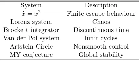
system are captured in Table1.1(borrowed from [16]). From this table, one can see that polynomial systems can show a very rich variety of dynamic behaviour. On the other hand, the table also depicts that polynomial systems maybe in general very difficult to study. Therefore, this class of system is considered in this thesis.

Table 1.1: _{Example of Polynomial Systems}

System Description ˙

x=x2 Finite escape behaviour Lorenz system Chaos

Brockett integrator Discontinuous time Van der Pol system limit cycles

Artstein Circle Nonsmooth control MY conjecture Global stability

[image:33.596.202.431.530.631.2]

(34)

Chapter 1. Introduction 19 designing the controller for polynomial discrete-time systems.

However, with the utilisation of state-dependent Lyapunov functions, the controller design for polynomial discrete-time systems becomes very difficult. This is due to the fact that the relation between the Lyapunov function and the controller matrix is no longer jointly convex. This problem will be highlighted in detail in Chapter 2. In continuous-time system, the aforementioned problem can be avoided by assuming that the Lyapunov matrix is only dependent upon the control input whose corresponding rows are zero [33]. Unfortunately, for discrete-time systems, although the same assumption is made, the problem still exists. A possible way to resolve this problem is given in [44], but the results suffer from some conservatism and such conservatism has been discussed earlier. In this thesis, we attempt to relax the problem by incorporating an integrator into the controller structures. In particular, we called this method as integrator method. Due to the problem that is discussed above, only a few results are available in the area of controller synthesis in the context of polynomial discrete-time systems [41,44]. As our discussion in the literature earlier shows, the results from both papers are suffering from their own conservatism. This consequently motivates us to carry out work on polynomial discrete-time systems stabilisation. Hence a more general and less conservative result can be provided than the available approaches.

Furthermore, it is also necessary for us to consider the robust controller design for poly-nomial discrete-time systems because to date, to the author’s knowledge, no results have been presented in this framework that consider the SOS programming technique. For this context, the polytopic uncertainty and norm-bounded uncertainty will be con-sidered because both of them are commonly appear in the real world. Besides, the norm-bounded uncertainty is not fully studied in the area of polynomial systems. This is another motivation that leads us to consider the norm-bounded uncertainty in our research work.

(35)

1.5

Contribution of the Thesis

The focus of this thesis is to establish novel methodologies for robust stabilisation, control with disturbance attenuation and filter design for a class of polynomial discrete-time systems. The polytopic uncertainties and norm-bounded uncertainties are considered in this research work and the proposed controller should able to handle the appearance of such uncertainties.

The main contribution arises from the incorporation of an integrator into the controller structures. In doing so, a convex solution to the polynomial discrete-time systems sta-bilisation with the utilisation of a state-dependent Lyapunov function function can be obtained in a less conservative way than the available approaches. In the light of this integrator method, the problem of robust control and robustH∞control for polynomial discrete-time systems are tackled. The integrator method is also applied to the filter design problem.

In this thesis, we first highlight the problem of the controller design for polynomial discrete-time systems when the state-dependent Lyapunov function is under consider-ation. Motivated by this problem, we propose a novel method in which an integrator is proposed to be incorporated into the controller structures. Then, we show that the original systems with the proposed controller can be described in augmented forms. In addition, by choosing the Lyapunov matrix to be only dependent upon the original sys-tem’s states, a convex solution to the robust control problem and robust H∞ control problem for polynomial discrete-time systems can be rendered in a less conservative way than available approaches.

In light of the integrator method, we propose a novel methodology for designing a robust nonlinear controller in which the polytopic and norm-bounded uncertainty are under consideration. It should be noted here that, to date, no result is available in this framework that utilises SOS programming for polynomial discrete-time systems. Furthermore, the interconnection between the nonlinear H∞ control problem and the robust nonlinear H∞ control problem is provided through a so-called ′

scaled′

systems. This allows us to efficiently solve the robust H∞ control problem with the existence of norm-bounded uncertainties. Next, we show that by exploiting the integrator method, a filter design methodology can also be established for polynomial discrete-time systems. Furthermore, by applying the integrator method, the output feedback controller is de-veloped for polynomial discrete-time systems with and without H∞ performance and also with and without uncertainties.

(36)

Chapter 1. Introduction 21 show that the proposed design methodologies can achieve the stability requirement or the prescribed performance index.

1.6

Thesis Outline

The contents of the thesis are as follows:

Chapter 2describes a nonlinear feedback controller design for polynomial discrete-time

systems. In this chapter, the problems of designing a controller for polynomial discrete-time systems are highlighted first. Then, a novel method for solving the problem is proposed. Furthermore, we show that the results can be directly extended to the robust control problem with polytopic uncertainty. The existence of the proposed controller is given in terms of the solvability of polynomial matrix inequalities (PMIs), which are formulated as SOS constraints and can be solved by the recently developed SOS solvers. The effectiveness of the proposed method is confirmed through a simulation example.

Chapter 3 demonstrates a robust nonlinear feedback controller design with the

exis-tence of norm-bounded uncertainties. We show that the uncertainties are tackled by applying an upper bound technique. The effectiveness of the proposed method is vali-dated through a demonstrative example.

Chapter 4presents a nonlinearH∞state feedback control for polynomial discrete-time

systems. TheH∞performance is needed to be fulfilled in this chapter while at the same time the system’s stability is guaranteed. A less conservative result than the available approaches is obtained through the utilisation of an integrator approach. The result is then directly extended to the robust nonlinear H∞ control problem with polytopic uncertainties. The sufficient conditions for the existence of the proposed controller is given in terms of the solvability of SOS inequalities and solved using SOSTOOLS. A tunnel diode circuit is used to demonstrate the validity of the proposed approach.

In Chapter 5, we study the robust nonlinear H∞ state feedback control for

polyno-mial discrete-time systems with the appearance of norm-bounded uncertainties in the system’s state and input. The ′

scaled′

system is introduced in this chapter, and the interconnection between the nonlinear H∞ control problem (described in Chapter 3) and the robust nonlinear H∞ control problem is established. We show that the ro-bust nonlinear H∞ control problem is solvable only if the ′

scaled′

(37)

Chapter 6deals with the problem of filtering design for a class of polynomial

discrete-time systems. By utilising the integrator method, a possible solution to the filter design problem is presented. Solutions to the filter design have been derived in terms of PMIs, which are formulated as SOS constraints. A numerical example is given along with the theoretical presentation.

In the above chapters, we assume that all the states are available for feedback which is not true in many practical cases. Therefore, inChapter 7we investigate the nonlinear

H∞ output feedback control for polynomial discrete-time systems. The problems of designing the output feedback controller are given in this chapter. Then, a novel method is proposed in order to overcome those problems. The results are then directly extended to the robustH∞ control problem with polytopic uncertainty. The sufficient conditions for the existence of such a controller is given in terms of the solvability of SOS inequalities and can be solved by the recently developed SOS solver.

InChapter 8, motivated by the results illustrated in Chapter5, we develop a

method-ology for robust controller design with H∞ performance with the existence of norm-bounded uncertainties. Again, in this chapter we show that the robust nonlinear H∞

control problem is solvable only if the ′ scaled′

system is solvable.

Concluding remarks are given and suggestions for future research work are discussed in

Chapter 8. Finally, some mathematical background knowledge that is used throughout

(38)

Chapter 2

Nonlinear Control for Polynomial

Discrete-Time Systems

2.1

Introduction

The controller design for polynomial discrete-time systems is a hard problem. This is due to the fact that the relation between the Lyapunov function and the controller matrix is always not jointly convex. In continuous-time systems, a convex solution can be achieved by restricting the Lyapunov function to be the only function of states whose corresponding rows in the control matrix are zeroes and whose inverse is of a certain form [32–34]. Unfortunately, this leads to the results being conservative. In discrete-time systems, the nonconvex problem remains persistent although the same restriction is applied. The attempt to design a state feedback controller for polynomial discrete-time systems can be found in [44]. The proposed methodology suffers from several sources of conservatism and such conservatisms have been discussed in the preceding chapter. Motivated by the results in [44] and the problem that has been mentioned above, this chapter attempts to convexify the state feedback control problem for polynomial discrete-time systems in a less conservative way and consequently leads to a less conservative controller design procedure for polynomial discrete-time systems. To be precise, in our work a less conservative design procedure is achieved by incorporating an integrator into the controller structure. In doing so, an original system can be transformed into an augmented system, and the Lyapunov function can be selected to be only dependent upon the original system states. This consequently causes the solution of controller synthesis for polynomial discrete-time systems to be convex and therefore can possibly be solved via SDP. It is important to note here that the resulting controller is given in terms of a rational matrix function of the augmented system. The sufficient condition

(39)

Chapter 2. Nonlinear Control for Polynomial Discrete-Time Systems 24 for the existence of our proposed controller is given in terms of the solvability condition of PMIs, which is formulated as SOS constraints. The problem, then, can be solved by the recently developed SOS solvers.

The rest of this chapter is organised as follows: Section 2.2 provides the main results in which the problem of designing a state feedback controller is highlighted first, then a novel method is proposed to overcome the problem. The results are then directly extended to the robust control problem with polytopic uncertainty. The validity of our proposed approach is illustrated using a simulation example in Section2.3. Conclusions are given in Section2.4.

2.2

Main Result

In this section, we present the robust nonlinear feedback controller design for polyno-mial discrete-time systems with an integrator. The significance of incorporating the integrator into the controller structure can be seen in this section. We begin this section by synthesising the controller without the existence of uncertainties, and the result is subsequently extended to the robust controller design with the existence of polytopic uncertainties.

2.2.1 Nonlinear feedback control design

Consider the following dynamic model of a polynomial discrete-time system:

x(k+ 1) =A(x(k))x(k) +B(x(k))u(k) (2.1) where x(k) _∈ Rn is a state vector and u(k) is an input. A(x(k)), and B(x(k)) are polynomial matrices of appropriate dimensions.

For system (2.1), the state feedback controller is proposed as follows:

u=K(x(k))x(k). (2.2) For this purpose, we use the standard assumption for the state feedback control where all states vector x(k) are available for feedback. The following theorem is established for the system (2.1) with the controller (2.2).

(40)

Chapter 2. Nonlinear Control for Polynomial Discrete-Time Systems 25

1. There exist a positive definite symmetric polynomial matrix, P(x(k)) and polyno-mial matrix,K(x(k)) such that

−(A(x(k)) +B(x(k))K(x(k)))TP−₁

(x+)(A(x(k)) +B(x(k))K(x(k)))

+P−₁

(x(k))>0, (2.3)

or

2. There exist a positive definite symmetric polynomial matrix, P(x(k)), polynomial matrices, K(x(k)) andG(x(k)) such that

"

GT(x(k)) +G(x(k))₋P(x(k)) _∗

A(x(k))G(x(k)) +B(x(k))K(x(k))G(x(k)) P(x+)

#

>0. (2.4)

Proof: Select a Lyapunov function as follows:

V(x(k)) =xT(k)P−₁

(x(k))x(k) (2.5) Then the difference of (2.5) along (2.1) with (2.2) is given by

∆V(x(k)) =V(x(k+ 1))₋V(x(k))<0 =xT(k+ 1)P−₁

(x+)x(k+ 1)−xT(k)P−1(x(k))x(k)

= A(x(k))x(k) +B(x(k))K(x(k))x(k)T

P−₁

(x+) A(x(k))x(k)

+B(x(k))K(x(k))x(k)

−xT(k)P−1

(x(k))x(k) =xT(k)

(AT(x(k)) +KT(x(k))BT(x(k)))P−1

(x+)(A(x(k))

+B(x(k))K(x(k)))₋P−1

(x(k))

x(k) (2.6)

Now we have to show that (2.4) _⇔ (2.3): (Necessity) Choose G(x(k)) = GT(x(k)) =

P(x(k)). (Sufficiency) Suppose (2.4) holds, thus GT(x(k)) +G(x(k)) > P(x(k)) > 0. This implies that G(x(k)) is nonsingular. Since P(x(k)) is positive definite, hence the inequality

(P(x(k))₋G(x(k)))T P−₁

(x(k)) (P(x(k))₋G(x(k)))>0 (2.7) holds. Therefore establishing

GT(x(k))P−₁

(41)

Chapter 2. Nonlinear Control for Polynomial Discrete-Time Systems 26 and therefore we have

"

GT₍_x₍_k₎₎_P−₁

(x(k))G(x(k)) _∗

A(x(k))G(x(k)) +B(x(k))K(x(k))G(x(k)) P(x+)

#

>0. (2.9) Next, multiply (2.9) on the right bydiag[G−1

(x(k)), I] and on the left by

diag[G−₁

(x(k)), I]T_{, we get}

"

P−1

(x(k)) _∗

A(x(k)) +B(x(k))K(x(k)) P(x+)

#

>0. (2.10) Applying the Schur complement to (2.10), we arrive at (2.3). Knowing that (2.3) holds, we have ∆V(x(k))<0,_∀x₆= 0, which implies that the system (2.1) with (2.2) is globally asymptotically stable. This completes the proof. ∆∆∆

Remark 2.2. The advantages of formulating the problem of the form (2.4) are twofold: 1. The Lyapunov function is decoupled from the system matrices. Therefore, the

selection of the polynomial feedback control law can be chosen to be a polynomial of arbitrary degree, which improves the solvability of the nonlinear matrix inequalities by the SOS solver. This also allows the method to be extended to the robust control problem.

2. The number of P(x(k)) can be reduced significantly in the problem formulation. The introduction of this new polynomial matrix method is first proposed in [60] for linear cases, and has been adopted by [44] for nonlinear cases. It is also important to note here that this new polynomial matrix,G(x(k)) is not constrained to be symmetrical.

It is worth mentioning that the conditions given in Theorem 2.1 are in terms of state dependent polynomial matrix inequalities (PMIs). Thus, solving this inequality is com-putationally hard because one needs to solve an infinite set of state-dependent PMIs. To relax these conditions, we utilise the SOS decomposition approach as described in [30] and have the following proposition:

Proposition 2.3. The system (2.1) is asymptotically stable if there exist a symmetric

polynomial matrix, P(x(k)), polynomial matrices L(x(k)) and G(x(k)), and constants

ǫ1>0 andǫ2 >0 such that the following conditions hold for all x6= 0

vT[P(x(k))₋ǫ1I]v is a SOS (2.11)

(42)

Chapter 2. Nonlinear Control for Polynomial Discrete-Time Systems 27 where,

M(x(k)) =

"

GT(x(k)) +G(x(k)₋P(x(k)) _∗

A(x(k))G(x(k)) +B(x(k))L(x(k)) P(x+)

#

(2.13)

Meanwhile,v and v1 arefreevectors with appropriate dimensions and

L(x(k)) =K(x(k))G(x(k)). Moreover, the nonlinear feedback controller is given by

K(x(k)) =L(x(k))G−₁

(x(k)).

Proof: The proof for this proposition can be obtained easily by following the technique

given in the proof section of Theorem 2.1. Then by Proposition 1.2 (given in Chapter 1), if the inequalities described in (2.11)-(2.12) are feasible, it implies that inequality (2.4) is true. The proof ends. ∆∆∆

Remark 2.4. Proposition 2.3 provides a sufficient condition for the existence of a state feedback controller and is given in terms of solutions to a set of parameterised poly-nomial matrix inequalities (PMIs). Notice that P(x+) appears in the PMIs,

there-fore the inequalities are not convex because P(x+) =P(x(k+ 1)) = P(A(x(k))x(k) +

B(x(k))K(x(k))x(k)). Therefore it is very difficult to directly solve Proposition2.3 be-cause the PMIs need to be checked for all combination of P(x(k)) andK(x(k)), which results in solving an infinite number of polynomial matrix inequalities. A possible way to resolve this problem has been proposed in [44] in which a predefined upper bound is used to limit the effect of the nonconvex term. However, this predefined upper bound is hard to determine beforehand, and the closed loop stability can only be guaranteed within a bound region. Motivated by this fact, we propose a novel approach in which the aforementioned problem can be removed by incorporating the integrator into the controller structure. This consequently provides a less conservative result on the similar underlying issue. The details of our method are given in the following text.

2.2.2 The integrator approach

In this section, we show that by incorporating the integrator into the controller struc-ture, the controller synthesis for polynomial discrete-time systems can be convexified efficiently and therefore a less conservative design procedure can be achieved.

The nonlinear feedback controller with the integrator is proposed as follows:

xc(k+ 1) =xc(k) +Ac(x, xc) u(k) =xc(k)

  

(43)

Chapter 2. Nonlinear Control for Polynomial Discrete-Time Systems 28 wherexc is an additional state or controller state. TheAc(x, xc) is an input function of

the integrator andu(k) is an input to the system. Here, the objective is to stabilise the system (2.1) with the controller (2.14).

The system (2.1) with the controller (2.14) can be described as follows: ˆ

x(k+ 1) = ˆA(ˆx(k))ˆx(k) + ˆB(ˆx(k))Ac(x, xc) (2.15)

where, ˆ

A(ˆx(k)) =

"

A(x(k)) B(x(k)) 0 1

#

; Bˆ(ˆx(k)) =

"

0 1

#

; xˆ(k) =

"

x(k)

xc(k)

#

; (2.16)

Next, we assumeAc(x, xc) to be of the formAc(x, xc) = ˆAc(ˆx(k))ˆx(k). Therefore (2.15)

can be re-written as follows: ˆ

x(k+ 1) = ˆA(ˆx(k))ˆx(k) + ˆB(ˆx(k)) ˆAc(ˆx(k))ˆx(k) (2.17)

where ˆA(ˆx(k)), and ˆB(ˆx(k)) are as described in (2.16). Meanwhile ˆAc(ˆx(k)) is a 1×(n+1)

polynomial matrix, where nis the original state number.

Remark 2.5. The above idea of introducing an additional dynamic is not new, see [61,62]. However, the authors in [61,62] used this method to overcome the problem of designing a robust controller for linear systems with norm-bounded uncertainties. In contrast, we propose this method