SPACES
T. BAKHTIAR1,SAMSURIZAL2, N. ALIATININGTYAS3
Abstract
It is well-known that in control theory the stability region of continuous-time system is laid in the left half plane of complex space, while that of discrete-time system is dwelled inside a unit circle. The former fact might be shown by exploiting the Laplace transform and the later by utilizing the corresponding zeta transform. In this paper we revealed the connectivity of both regions by employing M¨obius transform. We also used the same transform to derive continuous/discrete-time counterpart of several existing results, including Bode integral and Poisson-Jensen formula. We then demonstrated their unification property by using delta transform. Some numerical examples were provided to verify our results.
Keywords: continuous-discrete unification, M¨obius transform, delta transform, stability
1
INTRODUCTION
In control theory, some results for continuous-time and discrete-time such as regions of stability, expressions for minimum tracking error and energy regu-lation are derived independently. It is well-known that the stability region of continuous-time system is laid in the left hand side of imaginary axis in com-plex space, while that of discrete-time system is located inside a unit circle. In this paper, instead of using rigorous derivation we aim to utilize the strength of the M¨obius transform to obtain the counterpart of existing results, which cover the Bode integral and Poisson-Jensen formula.
While discrete system is obtained from continuous-time system by sam-pling, expressions in continuous and discrete domains are not quite clear. This is because the underlying continuous domain descriptions cannot be obtained by setting sampling period to zero in the discrete domain approximations. In optimal tracking error control problem, for instance, contribution of non-minimum phase zeros for continuous and discrete-time systems are provided in completely different ways, see [3, 7]. The delta operator has often been
1
Department of Mathematics, Bogor Agricultural University, Bogor. 2
Madrasah Aliyah Negeri 1, Bandar Lampung, Indonesia. 3
proven entailing many advantages in connecting discrete-time and continuous-time systems, such as control synthesis [4], control design [5], estimation [9] and filtering [11]. We then provide the delta domain version of some existing results.
2
REGION OF STABILITY
The most commonly used definitions of stability are based on the magnitude of the system response in the steady state. A system is said to be (asymptotically) stable if its response to any initial conditions decays to zero asymptotically in the steady state, otherwise is said to be unstable. From the perspective of the forced response of the system for a bounded input, a system is said to be bounded-input and bounded-output (BIBO) stable if its response to any bounded input remains bounded. This section reviews the region of stability for continuous-time and discrete-time systems.
2.1 Continuous-time System
Consider a linear continuous-time system given by an initial value problem of
n-th order differential equation:
n
X
i=0
aiy(i)(t) =
m
X
j=0
bju(j)(t), y(i)(0) =u(j)(0) = 0, (1)
wherey(t) andu(t) respectively are the output and input of the system,ai(i= 0, . . . , n) and bj (j = 0, . . . , m) are real coefficients, and an and bm are non-zeros. Note that in (1), y(i) denotes the i-th derivative of y with respect to time t. System (1) can be expressed in frequency domain, i.e., s-domain, by Laplace transform
n
X
i=0
aisiY(s) =
m
X
j=0
bjsjU(s),
where Y(s) := L{y(t)} and U(s) := L{u(t)} respectively denote the Laplace transform ofy(t) andu(t). The system possesses the following transfer function
H(s) = bms
m+b m−1sm
−1
+. . .+b1s+b0 ansn+an−1sn
−1
+. . .+a1s+a0
, (2)
where H(s) represents the transfer function between input U(s) and output
Y(s), i.e., Y(s) = H(s)U(s). If it is assumed that H has no zeros and poles in the same location, then we may write (2) as
H(s) = c(s−z1)(s−z2)· · ·(s−zm) (s−p1)(s−p2)· · ·(s−pn)
wherezj (j = 1, . . . , m) and pi(i= 1, . . . , n) are zeros and poles of H,
respec-tively, and cis a real constant. As we assume that n≥m, (3) can be written in term of partial fraction decomposition as follows,
H(s) =
By considering an impulse input function, i.e., U(s) = 1 or equivalently
u(t) =δ(t), then the time domain solution for (1) can be obtained by applying the inverse Laplace transform:
y(t) =
It can easily be seen from (5) that system (1) is (asymptotically) stable, i.e., limt→∞y(t) = 0, if and only if Repi < 0 for all i = 1, . . . , n. In other words, the stability region of continuous-time system is laid in the left half plane of complex space.
2.2 Discrete-time System
Consider a linear discrete-time system represented by a single n-th order dif-ference equation relating the output y to the inputu:
n version of system (6), i.e.,
n transform ofy(k) and u(k). Thus we have the following transfer function
H(z) = bmz rewritten as a power series
By applying the inverse zeta transform we have
y(k) =
k
X
i=0
ciu(k−i). (9)
Let |u(i)| ≤M for all i and C =P∞
i=0ci. Then,
|y(k)|=
k
X
i=0
ciu(k−i)
≤
k
X
i=0
|ci||u(k−i)| ≤M C
for each k = 0,1, . . .. Therefore the linear system (6) is stable. The proof of the converse can be found in [6]. As we completed the proof, it is shown that the stability region of a linear discrete-time system lies inside the unit circle.
3
M ¨
OBIUS TRANSFORM
It has been revealed in the previous section that the region of stability of continuous-time system is the left half plane of complex space, while that of discrete-time system is the interior of a unit circle. In this section we will utilize the M¨obius transform [2] to show the interconnection between these two regions. In particular, we demonstrate that the region of stability of discrete domain can be asserted by M¨obius transforming that of continuous domain.
Definition 1 (M¨obius Transform). Transformation
s=M(z) := az+b
cz+d, ad−bc6= 0, (10)
where a, b, c and d are complex-valued constants, is called M¨obius transform from variable z to variable s.
When c6= 0, equation (10) can be written
s = a
c +
bc−ad c
1
cz+d,
from which we can see that condition ad−bc6= 0 ensures that we do not have a constant function. If we assign M(∞) =∞ for c= 0, and M(∞) = a
c and
M(−dc) = ∞ for c 6= 0, then M¨obius transform (10) is certainly a bijective mapping of the extendedz-domain onto the extendeds-domain. When a given point s is the image of some point z under transformation (10), the point z is retrieved by its inverse
z =M−1
(s) := −ds+b
cs−a , ad−bc6= 0. (11)
We can verify that the inverse function (11) is also a bijective mapping by using the definition M−1
(∞) =∞ forc= 0, and M−1
(ac) = ∞andM−1
3.1 Region of Stability Mapping
In Section 2 the regions of stability for continuous-time and discrete-time sys-tems were derived separately by employing the Laplace and zeta transforms, respectively. In this part we will show that the region of stability for discrete-time system can be obtained by M¨obius transforming that for continuous-discrete-time system. To facilitate our analysis, for C the complex space we define the following sets: C−
:= {s ∈ C : Res < 0}, C+ := {s ∈ C : Res > 0}, D:={z ∈C:|z|<1}, Dc:={z∈C:|z| ≥1} and ¯Dc:={z ∈C:|z|>1}.
For the analysis we consider a special case of M¨obius transform where
a=c=d= 1 andb =−1, that is
The above is nothing but the modulo of complex numbers
|(α+ 1) +jβ|<|(α−1) +jβ| ⇔ |s+ 1|<|s−1|.
By applying (12) to above inequality we have
corresponds toz∈D, which reveals the interconnection between region of stability in s-domain and its counterpart in z-domain.
3.2 Other Continuous-Discrete Relationships
Now we further exploit the use of special M¨obius transform (12) to unveil the counterpart of existing continuous-time or discrete-time results, which covers Bode integral and Poisson-Jensen formula.
Theorem 2 (Bode integral in s-domain). Let g(s) be an analytic function in C+. Denote that g(jω) =g1(ω) +jg2(ω) and g(s) =g(¯s), i.e., g is conjugate
Theorem 3 (Bode integral in z-domain). Let f(z) be an analytic function in Equation (14) is claimed from (13) by substitution.
Theorem 4 (Poisson-Jensen formula in z-domain). Let f is analytic in D¯c and di(i = 1, . . . , nd) be the zeros of f in D¯c, counting their multiplicities. If
Proof. The Poisson-Jensen formula can be found in many standard books
on complex analysis. See for instance [1].
The continuous-time counterpart of Poisson-Jensen formula is provided as follows.
Theorem 5 (Poisson-Jensen formula in s-domain). Let g is analytic in C+ and ci (i = 1, . . . , nc) be the zeros of g in C+, counting their multiplicities. If
Proof. Perform transformation (12) over Theorem 4 to prove it.
4
DELTA TRANSFORM
A book that provides a comprehensive account on delta operator is [8]. The delta operator δ is define as the following forward difference
δ, q−1
whereqis the forward shift operator commonly used in discrete-time case and
By taking the zeta transform of above equation we obtain
δX(z) = z−1
T X(z).
We may say that inz-plane the delta operator will translate a pointz ∈Cone unit to the left and then scale it by factor of 1
T. Later, the variable δ is used
as the delta operator variable and is analogous to the Laplace variable s for continuous-time systems and the zeta transform variable z for discrete-time systems. We then obtain the relationship between variablez and variableδ as follows,
δ= z−1
T ⇔z =T δ+ 1. (17)
For any sequencex(k) we define its delta transform by
D{x(k)}=XT(δ) :=T
Now we ready to present the δ-domain counterparts of previous theorems. For time samplingT we define the following sets: DT :={δ ∈C:|T δ+1|<1}, Dc
T :={δ∈C:|T δ+ 1| ≥1} and ¯DcT :={δ∈C:|T δ+ 1|>1}.
Theorem 6 (Bode integral in δ-domain). Let h be an analytic function in Dc
easily verify thath′
(0) =T f′
(1),dθ =T dωand{z =ejθ} 7→ {δ=e(jωT−1)/T
}. Theorem 7 (Poisson-Jensen formula in δ-domain). Let h is analytic in D¯c
5
NUMERICAL EXAMPLE
In this section we provide a simple illustrative example to verify our result and to show the unification property between δ-domain and s-domain results.
5.1 Verification
To verify the result presented in Theorem 3 we consider a function f defined in z-domain as follows,
f(z) = 3z+ 1
z−p , −1< p <1. (20)
Since pole p lies inside the unit circle, indeedf is analytic in Dc and it can be written as f(ejθ) =f
1(θ) +jf2(θ), where
f1(θ) = 3−p+ (1−3p) cosθ
p2−2pcosθ+ 1 ,
f2(θ) = −
(1 + 3p) sinθ p2−2pcosθ+ 1.
Further, the LHS of (14) is given by
2f′
(1) =−2(3p+ 1)
(p−1)2 . (21)
Whereas, for the RHS we have
1
π Z π
−π
f1(θ)−f1(0) 1−cosθ dθ
= 1
π Z π
−π
3−p+(1−3p) cosθ
p2−2pcosθ+1 − 4 1−p 1−cosθ dθ
= (p+ 1)(3p+ 1)
π(p−1)
Z π
−π
dθ
p2−2pcosθ+ 1. (22)
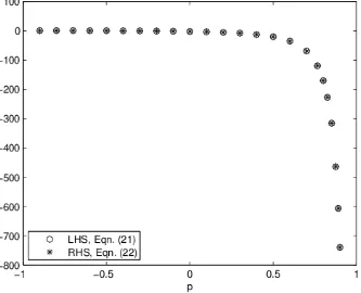
Figure 1: Bode integral in z-domain
5.2 Unification
Sinceg(s) =f(1+1−ss), from (20) we obtain
g(s) = 4 + 2s
(1 +p)s+ 1−p, (23)
from which we also have
g′
(0) =−2(3p+ 1) (1−p)2 .
In the δ-domain, from the relationship h(δ) = f(T δ+ 1) we have
h(δ) = 3T δ+ 4
T δ + 1−p, (24)
and thus
h′
Therefore, the unification property of Theorems 2, 3 and 6 is unveiled by fact that
lim
T→0 2h′
(0)
T = limT→0−
3T p+T T(1−p)2 =−
3p+ 1 (1−p)2 =g
′ (0),
which show that the LHS of (18) converges to that of (13) as the sampling time T decreases.
6
CONCLUDING REMARK
It has been shown that M¨obius transform can be utilized to derive counterpart result without involving any rigorous derivation. The delta transform, which takes a time sampling into account, can be used to show the unification prop-erty between continuous and discrete results. The approach describes in this paper can then be exploited to derive many more counterpart expressions.
References
[1] Ash RB, Novinger WP. 2007.Complex Variables. 2nd Ed. Dover.
[2] Brown JW, Churchill RV. 2009.Complex Variables and Application. 8th Ed. McGraw-Hill.
[3] Chen G, Chen J, Middleton R. 2002. Optimal tracking performance for SIMO systems. IEEE T. Automat. Contr.47(10):1770–1775.
[4] Collins EG. 1999. A Delta Operator Approach to Discrete-time H∞ Control. Int. J.
Control. 72(4):315–320.
[5] Emami T. 2007. A Unified Procedure for Continuous-Time and Discrete-time Root-Locus and Bode Design.Proc. Amer. Contr. Conf.pp 2509–2514.
[6] Fisher SD. 1999.Complex Variables. 2nd Ed. Dover.
[7] Hara S, Bakhtiar T, Kanno M. 2007. The Best AchievableH2 Tracking Performances for SIMO Feedback Control Systems. J. Contr. Sci. Eng. pp 1–12.
[8] Middleton RH, Goodwin GC. 1990. Digital Control and Estimation: A Unified Ap-proach. Prentice Hall.
[9] Ninness BM, Goodwin GC. 1991. The Relationship Between Discrete Time and Con-tinuous Time Linear Estimation,” in Sinha, N.K. and Rao, G.P. (Eds). Identification of Continuous-Time Systems, International Series on Microprocessor-Based Systems Engineering. 7:79–122.
[10] Seron MM, Braslavsky JH, Goodwin GC. 1997.Fundamental Limitations in Filtering and Control. Springer.