DETERMINING POVERTY MAP
USING SMALL AREA ESTIMATION METHOD
Abstract. Poverty is a phenomenon that always occurs in every country especially in the
developing country such as Indonesia. Poverty is defined as a condition where someone has not capability to fulfill their basic needs (food and non food). The difference of geographic condition and the unequal of demography always become some problems in the geographic targeting of the poor in the poverty reduction program. One of method that is accurately effective and sensitive with poverty in the small area is Small Area Estimation method by Elbers et al. It is known as Elbers, Lanjouw, Lanjouw method (ELL method). The objective of this method is to map the incidence of poverty in every county or city using the steps in ELL method. In this study, we use Central Java as our case study. The results of this study are the model consumption of Central Java, poverty indicators for each city in Central Java and the poverty maps so that can give information and facilitate the government for making priority in poverty reduction programs.
Keywords: Poverty map, ELL Method
1. INTRODUCTION
Poverty is a phenomenon that always occurs in every country especially in the
developing country. Every country has the difference of geographic condition, poverty
levels, the tools to measure and handling the poverty. Poverty is defined as a condition
where someone has not capability to fulfill their basic needs (food and non food).
Someone is called as a poor people if his or her expenditure or income below poverty
line. Poverty line is the minimum incomes that have to fulfill his or her minimum living
standard. If poverty line is high, then there are so many people that are poor.
Indonesia, a country that is very large in size of population and has the difference
of geographic condition in every province, always has some problems in the geographic
targeting of the poor in the poverty reduction program. Obviously, in order to make
poverty reduction programs, we need an instrument that is accurately effective and
sensitive with poverty, which in turn the objective of poverty reduction can be exactly
attained.
SMERU [7] stated that, ideally, geographic targeting should be based on a
description of poverty incidence and other indicators of economic welfare in small area or Eko Yuliasih and Irwan Susanto
Determining Poverty Map Using Small Area Estimation Method FMIPA UNS at low administrative levels. In Indonesia, the administrative levels start from the national
level, and descend to the provincial, county or city, sub district, and village levels.
There is one way to obtain village level information on the distribution of
economic welfare that is to carry out a household survey representative at the village
level. However, this is very difficult to be done because a household survey is too large
and expensive to carry out.
Fortunately, as a result of recent methodological advances in this study, the World
Bank has developed a new method to estimate small area distribution of economic
welfare from statistical data collections that is normally available in a country. The result
of this method will be pointed out in a geographic map, known as a poverty map.
A poverty map is a visual representation of the spatial incidence of poverty that can
facilitate the focused pro poor interventions and guide the allocation of public spending to
reduce poverty. It will help the government to reduce poverty exactly. Moreover, it can
reduce the risk of poor households being missed by poverty reduction programs.
One of the methods for producing small area estimation of the spatial description
of economic welfare is small area estimation method by Elbers, Lanjouw, Lanjouw. It is
known as Elbers, Lanjouw, Lanjouw (ELL) Method. This method was introduced by
Chris Elbers, J. O. Lanjouw, and Peter Lanjouw and is based on regression models of
income or expenditure with random effects at the level of survey clusters. This method
has been done successfully in other countries, especially in South Africa and Ecuador. In
the first application, this method would be done if the sources of data needed are
available. This method has been applied in Indonesia to map the poverty in East
Kalimantan, East Java and Jakarta. But no one has mapped the poverty in Central Java.
In this study, we use the application of small area estimation method that is
described by Elbers, Lanjouw, Lanjouw (or ELL method) to estimate the small area of
poverty in county or city levels, to calculate the poverty indicators, to make a poverty
map of Central Java and to interpret it.
2. THEORETICAL AND METHODOLOGY
2.1 The definition of poverty
According to the World Bank [2], poverty is concerned with absolute standard
living part of the poor society in the equality refers to relative living standards across the
Determining Poverty Map Using Small Area Estimation Method FMIPA UNS United Nations Development Program (UNDP) [2] defines poverty as hunger;
poor of haven; incapacity to go to a doctor when getting sick; have not any access to go to
school and illiteracy; jobless; afraid of the future; incapacity to get pure water; powerless;
has no representative and freedom.
According to Government’s Law No. 42 1981 [2], the poor is the people who
have not any job and have not any capability to fill their basic commodities of humanity
or people who have a job but they cannot fill the basic commodities of humanity. In
addition, by the Asian Development Banks’ point of view [2], poverty is a deprivation of
essential assets and opportunities that every human is entitled.
2.2 The indicators of poverty
In this study, we use poverty indicators from BPS. To measure poverty, BPS
calculates a number of summary statistics describing the incidence, depth and severity of
poverty. These include the headcount index (which measures the incidence of poverty),
the poverty gap (which measures the depth of poverty) and the poverty severity (which
measures the severity of poverty).
Foster, et al in Avenzora [1] show that the three poverty measures may all be
calculated using the following formula:
1
1
Mch
h
z y P
N z
, where
0,1, 2
(2.1)
where:
z= poverty line
ch
y = per capita consumption of household in location c
N= the number of people in the sample population
M = the number of poor people (household)
i. the headcount index. When
0, then0
0
1 1
1
1
1
.
M M
ch
h h
z y M
P
N z N N
Determining Poverty Map Using Small Area Estimation Method FMIPA UNS Commonly, it is denoted as the headcount ratio or when turned into a percentage, the
headcount index (proportion of person whose expenditure level is under the poverty
line). Although it is to interpret the incidence of poverty, the headcount index is not
sensitive to estimate how far below the poverty line poor people is.
ii. the poverty gap index. When
1, then1 1 1 1
1
1
.
M M ch ch h hz y z y
P
N z N z
(2.3)It is denoted as the poverty gap index which is simply the sum of all the poverty gaps
in the population can be used as an indicator of the minimum cost of eliminating
poverty using perfectly targeted transfers.
iii. the poverty severity index. When
2, then2 2 1
1
.
M ch h z y PN z
(2.4)This is poverty severity index which is sensitive to the distribution of living standards
among the poor. The poverty severity index measures the severity (or intensity) of
poverty. This is the other relevant poverty indicator that is inequality in the
distribution of expenditures among poor people (it is also referred to as severity).
To determine whether poverty has changed over time or varies over some
geographic or demographic characteristic, estimation of the sampling variance for the
indexes are required. According to Kakwani in Jollife [4], there are two formulas to
estimate the variance of the index class of poverty indexes that are easy to calculate the
frequent used. Those are
a. variance of P0
0
0
01
var
1
P P P n
, (2.5)Determining Poverty Map Using Small Area Estimation Method FMIPA UNS b. Variance of P,
1, 2
2 2
var
1
P P Pn
.(2.6)
2.3 The poverty mapping
Poverty map is a visual presentation of the spatial incidence of poverty able to
facilitate a better or a better focused pro poor interventions and guide the allocation of
public spending to reduce poverty. This poverty map will help the government in
reducing poverty precisely. Moreover, it can reduce the risk of poor households being
missed by poverty reduction programs.
According to Peter Lanjouw [5], there are three basic steps of poverty mapping.
Those are
Steps 1: identifying variables at the household level that is defined in the household
survey.
Steps 2: estimating model of consumption. The parameter estimates the model of
consumption and it will be applied to the census data, the expenditure is predicted and the
poverty statistics are derived.
Steps 3: inputting the model of consumption into census data at the household level, and
the estimation of poverty and inequality measure at a variety of levels of spatial
disaggregating.
2.4 Small Area Estimation
Small Area Estimation (SAE) [6] is a statistical technique that models the living
standard information available in small household survey data to establish comparability
of other non comparable household surveys with population census and generate
estimation of living standards of household in population census. SAE provides an
opportunity to obtain high resolution poverty maps through the integration of census data.
One of the methods for producing small area estimation of the spatial description
of economic welfare is small area estimation method by Elbers, Lanjouw, Lanjouw. It is
known as Elbers, Lanjouw, Lanjouw (ELL) method.
2.5 ELL method
ELL method [3] is a new method in the construction of poverty map that has been
introduced by the World Bank. This methodology is introduced by Chris Elbers, J. O.
Determining Poverty Map Using Small Area Estimation Method FMIPA UNS data sources. This method has capability to estimate the poverty level and the poverty
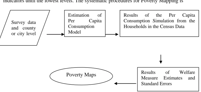
indicators until the lowest levels. The systematic procedures for Poverty Mapping is
Figure 1. Systematic Procedurs for Poverty mapping
2.6 The consumption model
According to Elbers et al [3], the first stage begins with an accurate empirical
model ofych, per capita expenditure of household hin locationc, is defined as:
ln
ych
xch
uch. (2.7) Whereln
ych is the logarithm of per capita consumption of household hin locationc,ch
x is a vector of characteristics of this household, and uch is the error term which is
distributedN
(0, )
.Because survey data is just a sub sample of whole population, the location
information is not available for all regions in the census data. Thus, we cannot include the
location variable in the survey model. Therefore, the residual of (2.7) must contain the
location variance and uch can be decomposed into uncorrelated terms:
ch c ch
u
. (2.8)Where
c is a location error term common to all household within the location and
ch isa household specific error term. It is further assumed that the
c is uncorrelated acrosslocation and the
ch is uncorrelated across households. With these assumptions, equation(2.7) is reduced to
lnychxch
c ch (2.9)Survey data and county or city level variables
Estimation of Per Capita Consumption Model
Results of the Per Capita Consumption Simulation from the Households in the Census Data
Results of Welfare Measure Estimates and Standard Errors
Determining Poverty Map Using Small Area Estimation Method FMIPA UNS
3. THE RESULT 3.1 Description Data
In this study, we use three sources of data: (i) SUSENAS 2006, (ii) Central Java in
Figure 2006, and (iii) data and information of poverty 2005-2006. To estimate the
consumption model, we use the data on household consumption obtained from
SUSENAS 2006, the data on household characteristics is obtained from Central Java in
Figure 2006 and to calculate the poverty measures, we use data and information of
poverty 2005-2006.
3.2 Selecting Variables.
The procedure in selecting the explanatory variables of equation (2.9) refers to
the research of SMERU and available in SUSENAS data. The explanatory variables are
only selected and will be used in estimating the consumption model if they contribute
significantly to the explanation of (log) per capita consumption. The explanatory
variables that are selected by stepwise method are occupation sector of household head
(agriculture and mining), household size and working status of household head (seeking).
3.3 Estimating the Consumption Model.
The result of 3.2 can give us information that explanatory variables will be used to
estimate the consumption model. First step to estimate the consumption model is to use
Ordinary Least Squares (OLS) and save the residuals as a variable ch
u
. We find the
consumption model as
6 6 5
ln
ych
14.127 0.4
a
(3.555 10 )
b
(1.728 10 )
c
(1.888 10 )
d (3.1) wherea = Household size
b = Working status of household head (seeking)
c= Occupation sector of household head (agriculture)
d= Occupation sector of household head (mining)
3.4 Calculating the Poverty Indicators.
There are three measurements of poverty indicators. These are the headcount
index which measures the incidence poverty, the poverty gap index which measures the
Determining Poverty Map Using Small Area Estimation Method FMIPA UNS Commonly, those poverty indicators are known as FGT family of poverty measures.
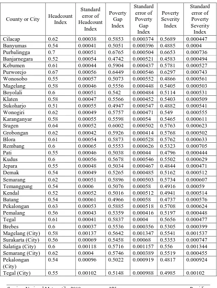
Using PovMap 2.0 [8], we find those poverty indicators for each location,
Table 3.1 The poverty indicators and standard errors of each poverty indicators for each
location
County or City Headcount Index Standard error of Headcount Index Poverty Gap Index Standard error of Poverty Gap Index Poverty Severity Index Standard error of Poverty Severity Index Cilacap 0.62 0.00038 0.5853 0.000374 0.5689 0.000447 Banyumas 0.54 0.00041 0.5051 0.000396 0.4885 0.0004 Purbalingga 0.7 0.00051 0.6765 0.000504 0.6653 0.000736 Banjarnegara 0.52 0.00054 0.4742 0.000521 0.4583 0.000494 Kebumen 0.61 0.00044 0.5904 0.000437 0.5781 0.000527 Purworejo 0.67 0.00056 0.6449 0.000546 0.6297 0.000743 Wonosobo 0.55 0.00057 0.5073 0.000552 0.4866 0.000561 Magelang 0.58 0.00046 0.5556 0.000448 0.5405 0.000503 Boyolali 0.6 0.00051 0.542 0.000484 0.5114 0.000531 Klaten 0.58 0.00047 0.5566 0.000452 0.5403 0.000509 Sukoharjo 0.51 0.00055 0.4947 0.000547 0.4882 0.000541 Wonogiri 0.62 0.00049 0.5757 0.000471 0.549 0.000555 Karanganyar 0.58 0.00055 0.5598 0.00054 0.5465 0.000611 Sragen 0.64 0.00052 0.6002 0.000502 0.5763 0.000623 Grobongan 0.62 0.00042 0.5926 0.000414 0.5768 0.000502 Blora 0.61 0.00054 0.5873 0.000528 0.5762 0.000633 Rembang 0.6 0.00065 0.5553 0.000626 0.5323 0.000705 Pati 0.55 0.00046 0.5038 0.00044 0.4796 0.000444 Kudus 0.6 0.00056 0.5678 0.000546 0.5502 0.000629 Jepara 0.55 0.00048 0.5034 0.000467 0.4844 0.000471 Demak 0.54 0.00049 0.5265 0.000485 0.5162 0.000512 Semarang 0.62 0.00051 0.5896 0.000503 0.5734 0.000607 Temanggung 0.54 0.0006 0.5076 0.00058 0.4916 0.00059 Kendal 0.52 0.00052 0.5016 0.000512 0.4941 0.000514 Batang 0.54 0.00061 0.4966 0.00058 0.4737 0.000576 Pekalongan 0.63 0.00053 0.5885 0.000518 0.5708 0.000624 Pemalang 0.56 0.00043 0.5359 0.000416 0.5197 0.000448 Tegal 0.61 0.00041 0.5837 0.0004 0.5656 0.000477 Brebes 0.6 0.00037 0.5536 0.000356 0.5305 0.000399 Magelang (City) 0.58 0.00137 0.5642 0.001347 0.5541 0.001537 Surakarta (City) 0.56 0.00069 0.5458 0.00068 0.5353 0.000747 Salatiga (City) 0.6 0.00118 0.5716 0.001157 0.556 0.001344 Semarang (City) 0.62 0.0004 0.5746 0.000389 0.5519 0.000455 Pekalongan
(City)
0.54 0.00096 0.5022 0.000919 0.4817 0.000924
Determining Poverty Map Using Small Area Estimation Method FMIPA UNS Table 3.1 provides the headcount index, poverty gap index, and poverty severity
index for each location. Let us see Cilacap, the headcount index of Cilacap is 0.62 or 62
% with standard error 0.00038. It means that there are 62% of people in Cilacap are poor.
Poverty gap index of Cilacap is 0.5853 or 58.53, it means that the gap between the
average gap of expenditure for every people and poverty line. The standard error of
poverty gap index is about 0.000374. Whereas poverty severity in Cilacap is 0.5689 or
56.89% with standard error 0.000447. It means that the severity in Cilacap is 56.89%.
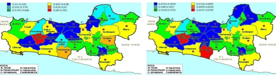
3.5 Poverty Maps of Central Java and The Interpretation.
Poverty map is a visual presentation of the spatial incidence of poverty that can
facilitate a better focus pro poor interventions and guide the allocation of public spending
to reduce poverty. Since the poverty indicators at county or city levels have been
calculated and available for each poverty indicator, we can make poverty maps for each
poverty indicators. These are the maps by virtue of poverty measures in every county or
city
Figure 3.1 Poverty Map by virtue of headcount
index
Figure 3.2 Poverty map by virtue of poverty
gap index
Figure 3.3 Poverty Class by Virtue of Poverty
Severity Index
In the calculation of poverty map, the poverty map is not only influenced by
Determining Poverty Map Using Small Area Estimation Method FMIPA UNS the county of Sukoharjo, for the incidence of poverty; it is in the interval of 0.51-0.542
where it is included in the lowest poverty incidence. It means that the poor people in
Sukoharjo are about 51% until 54.2%. For the poverty gap; it is in the interval of
0.4742-0.5079 where it is included in the lowest poverty gap index. It means that the gap
between the average gap of expenditure for every people and poverty line is about
47.42% until 50.79% and for the severity poverty; it is in the interval of 0.4583-0.4928
where it is included in the lowest poverty severity index or the severity level in county of
Sukoharjo is about 45.83% until 49.28%.
To interpret the other location, we can use the same interpretation on Sukoharjo.
Using the poverty poverty maps, we can make the priority in poverty reduction program.
4. The Conclusions
As mentioned in the previous chapter, we will conclude that
1. The estimation of consumption model is
6 6 5
ln
ych
14.127 0.4
a
(3.555 10 )
b
(1.728 10 )
c
(1.888 10 )
d wherea = Household size
b = Working status of household size
c= Occupation sector of household head (agriculture)
d= Occupation sector of household head (mining)
2. Using the consumption model of Central Java, we have calculated the poverty indicators (headcount index, poverty gap index, poverty severity index) and made
poverty maps by virtue of poverty indicators
BIBLIOGRAPHY
[1] Avenzora, A., Kemiskinan, Data dan Informasi Kemiskinan Tahun 2005-2006 Buku 2: Kabupaten (Data and Information of Poverty 2005-2006 2nd Book:
County), CV.Nario Sari, Jakarta, 2007.
[2] Asrial, Pemetaan Kemiskinan Kabupaten Gayo Lues 2005, Laporan Akhir, Badan Perencanaan Pembangunan Daerah Kabupaten Gayo Lues working wih
Badan Pusat Statistik Kabupaten Aceh Tenggara. Aceh Tenggara, Gayo Lues,
Determining Poverty Map Using Small Area Estimation Method FMIPA UNS [3] Elbers, C., et al, Micro-Level Estimation Poverty and Inequality. Econometrica,
2003,Vol. 71, No.1, 355-364.
[4] Jolliffe, D. (2003). Comparisons of Metropolitan-Nonmetropolitan Poverty During the 1990s. Rural Development Research Report Number 96. United States Department of Agriculture. United States America.
[5] Lanjouw, P., Estimating Geographically Disaggregated Welfare Levels and Changes, Tool Kit-Chapter 4. The World Bank.
[6] Rao, J.N.K., Small Area Estimation, a John Wiley&Sons, Inc, Publication, New Jersey, 1937.
[7] SMERU, Peta Kemiskinan Indonesia: Asal Mula dan Signifikansinya(The Poverty Map of Indonesia: Genesis and Significance), Newsletter No. 26: May-Aug/2008. Jakarta.
[8] Zhao,Q. and Lanjouw, P., Using PovMap2 A USER’s GUIDE. The World Bank,