A Quasi-Gaussian Kalman Filter
Suman Chakravorty, Mrinal Kumar and Puneet Singla
Abstract— In this paper, we present a Gaussian approxi-mation to the nonlinear filtering problem, namely the quasi-Gaussian Kalman filter. Starting with the recursive Bayes filter, we invoke the Gaussian approximation to reduce the filtering problem into an optimal Kalman recursion. We use the moment evolution equations for stochastic dynamic equations to evaluate the prediction terms in the Kalman recursions. We propose two methods, one based on stochastic linearization and the other based on a direct evaluation of the innovations terms, to perform the measurement update in the Kalman recursion. We test our filter on a simple two dimensional example, where the nonlinearity of the system dynamics and the measurement equations can be varied, and compare its performance to that of an extended Kalman filter.
I. INTRODUCTION
In this paper, we present a Gaussian approximation to the exact nonlinear filtering problem, namely the quasi-Gaussian Kalman filter. We consider a problem with continuous time state dynamics and discrete measurement updates. We use a Gaussian approximation to the nonlinear filtering problem in order to reduce the problem of nonlinear filtering to one of maintaining the estimates of the first two moments of the state variable based on the observations, i.e., an optimal Kalman recursion. We use the moment evolution equations for stochastic dynamical systems in order to evaluate the prediction terms in the nonlinear filtering recursions. Then, we propose two methods, one based on stochastic lineariza-tion and another based on direct evalualineariza-tion, to evaluate the innovations terms. We test the proposed filter on a simple two dimensional example, where the nonlinearity of the system dynamics and the measurement equations can both be varied, and compare its performance to that of an extended Kalman filter (EKF).
Nonlinear filtering has been the subject of intensive re-search ever since the publication of Kalman’s celebrated work in1960[1]. It is known that the solution to the general nonlinear filtering problem results in an infinite dimensional filter, in the sense that an infinite system of differential equations need to be solved in real time in order to solve the filtering problem exactly [2]–[5]. Hence, the nonlinear filtering problem is computationally tractable only if we con-sider finite dimensional approximations of the true infinite
Suman Chakravorty is with Faculty of Aerospace Engi-neering, Texas A&M University, College Station, TX, USA. [email protected]
Mrinal Kumar is a Graduate Assistant Research in Dept. of Aerospace Engineering at Texas A&M University, College Station, USA. [email protected]
Puneet Singla is a Graduate Assistant Research in Dept. of Aerospace Engineering at Texas A&M University, College Station, USA. [email protected]
dimensional filter [6]–[10]. However, even these methods are difficult to implement because of the complicated nature of the involved computations.
based on stochastic linearization and the other based on direct evaluation of the measurement update terms, in order to evaluate the innovations terms in the optimal recursions, i.e., to linearize the measurement equations. Our method does not require the choice of a set of sigma points and thus, is free from this design aspect. However, central to the implementation of our filter is the evaluation of integrals of the form of a product of a function and a Gaussian function. In the case of polynomial nonlinearities, these are the higher order moments of a Gaussian random variable. The rest of the paper is organized as follows.
In section 2, we introduce the Bayes filter. In section 3, we discuss the topic of Gaussian approximations in nonlinear filtering problems and present the optimal Kalman recur-sions. In section 4, we present our quasi-Gaussian Kalman filter and the methods we use to evaluate the optimal terms in the Kalman recursions for the approximate nonlinear filtering problem. In section 5, we present a two dimensional example, with variable nonlinearity in both system dynamics and measurement, and compare the performance of our filter with that of an EKF. In section 6, we present our conclusions and directions for further research.
II. BAYESFILTER
In this section, we introduce the recursive Bayes filter. Consider a system whose dynamics are governed by the Stochastic Ito differential equation,
dx=f(x)dt+g(x)dW, (1)
whereW represents a standard Wiener process. The system state is measured in a discrete fashion according to the equation,
yk =h(xk) +vk, (2)
wherevk is the measurement noise at instantk. Let Fk = {y0,· · · , yk} denote the history of the observations till the
time instant k. Then, the Bayes filter recursively updates the probability density of the state variable according to the following equations:
)represent the probability density of the system state at the kth
time instant, based on observations till the time instants k and (k−1) respectively, P(xk/xk−1)
represents the transition probability from statexk−1to state
xk corresponding to equation (1), and p(yk/xk) represents the probabilistic observation model corresponding to the observation equation (2). The prediction step in the Bayes filter, i.e. Eq.(3) makes use of the Chapman-Kolmogorov equations [22] for propagation in between measurements, while the update step (Eq. (4)) utilizes the Bayes rule. Note that in general, evaluating the multi-dimensional integral in the above equations is a formidable challenge. The predicted probability density function, p(xk/Fk−1
), can also be
ob-tained by solving the Fokker-Planck-Kolmogorov equation [22] corresponding to Eq.1, given by:
∂p
whereQrepresents the intensity of the Wiener process W. Now let
whereLF P denotes the differential operator corresponding to the Fokker-Planck-Kolmogorov equation. Thus, the integral in the Bayes filter corresponding to the prediction equation (Eq.3) can be evaluated by solving the above partial differ-ential equation. The prediction step in the Bayes filter can be solved by either evaluating the integral in the prediction equation through a Monte-Carlo type method (the subject matter of particle filters [23]) or by solving the above partial differential equation. However, solving the Fokker Planck equation is a tough proposition.
III. GAUSSIANAPPROXIMATIONS INNONLINEAR FILTERING
One method for obtaining a finite dimensional approx-imation to the infinite dimensional filter corresponding to a general nonlinear filtering problem is to approximate the state, the noise and the observation terms as Gaussian random variables. The Bayesian recursion shown above can then be greatly simplified, since the posterior distribution of the state always remains Gaussian under these approximations. Thus, estimates of only the conditional mean, E(xt/Ft), and covariance,Px need to be maintained. It can be shown that under the Gaussian approximation, we obtain following recursive filter [4], [13]:
¯
k andxk¯ represent the predicted and updated values of the mean of the random vectorxk,P−
xk, andPxkrepresent
the predicted and the updated values of the covariance matrix ofxk,Pykis the covariance matrix of the observationykand
Pxkyk is the cross-covariance matrix between the state and
observation. The key to implementing the above recursion is to evaluate the quantitiesx¯−
k,Px−k,Pyk andPxkyk. Different
filters use different ways to evaluate these quantities. In the EKF, the predicted mean and covariance of the variablexk are evaluated by linearizing the system dynamics about the previous estimatexk−1 and using linear Gaussian
analysis to propagate the mean and the covariance, while the quantities Pyk and Pxkyk are evaluated by linearizing
the measurement equation about the current predicted value ofxk and using linear Gaussian analysis.
[17], [20]. The sigma point filters perform linearization of the system dynamics and the measurement equations in a statistical sense as opposed to the Jacobean linearization which is performed in the case of the EKF.
In our approach, we adopt a different approach to eval-uate the prediction and innovation terms in the filtering recursions. We first use the moment evolution equations for the stochastic dynamical system along with the Gaussian approximation, and then perform a stochastic linearization of the measurement equation in order to evaluate the innovation terms. The details of the method are presented in the next section.
IV. A QUASI-GAUSSIANKALMANFILTER
In this section, we present our approach to nonlinear filtering based on Gaussian approximations of the prediction and innovation terms. As mentioned previously, we use the moment evolution equations for the prediction step. Then we propose two methods to evaluate the innovation terms: (a) stochastic linearization to linearize the measurement equations and (b) a direct method to evaluate the innovations terms.
A. Prediction
Recall the nonlinear filtering equations (7)-(9), and note that:
∂p
∂t =LF P(p), (10)
where LF P is the spatial operator of the Fokker Planck equation. We shall now find the time evolution equations for the first and second moments of the state variable, given the prior probability distribution. Let the prior probability distribution at the kth instant be given by N(¯xk, Px
k) and
the mean and the correlation of the state between the time instants bex¯ andRx respectively. By definition, we have:
¯
Then, it follows that the first and second moments ofxevolve according to the following differential equations:
˙¯
with the initial conditions xk¯ and Rxk respectively. The
above equations are integrated between thekthand(k+1)th time instants. In absence of the Gaussian approximation, the evaluation of the right hand side of the above equation involves higher moments of the random variablexbecause of the Fokker Planck operator. Due to the complicated nature of this operator, the above equations are difficult to handle. We present below an alternate method for deriving the moment evolution equations, and also the evolution equations of the correlation of the state x and its mean. Consider again the system equation (1) and an infinitesimal change in the
correlation of the statex,dE(xxt)
, given by:
dE[xxt] =E[(x+dx)(x+dx)t]−E[xxt].
(14)
Letdx=y, and recall the following definitions:
E[(x+y)(x+y)t] =
where p(x, y) represents the joint distribution function of the random variables x andy, and Eq.16 follows from the definition of conditional probability. Thus we have:
dE[xxt] =
Z
(xyt+yxt+yyt)p(x, y)dxdy.
(17)
It can be shown after some work that the following equations hold:
Using Eqs.18-19 in Eq.17, we obtain the following relation:
dE[xxt] = (E[xft(x)] +E[f(x)xt] +
E[g(x)Qgt(x)])dt+ (E[f(x)ft(x)])dt2
(20)
Dividing bydtand neglecting theO(dt)term leads us to the following evolution equations:
˙
E(xxt) = ˙Rx=E[xft(x)] +E[f(x)xt] +E[g(x)Qgt(x)],
˙
E(x) = ˙¯x=E[f(x)]. (21)
The initial conditions for the above equations are(¯xk, Rxk).
Following the Gaussian approximation, we substitutep(x) =
N(¯x, Rx). Further, if the functionsf andg are polynomials or can be well approximated by them, the right hand sides involve evaluation of the higher order moments of the (Gaussian) state vectorx.
B. Measurement Update
In this section, we present two methods for evaluating the innovations terms in the nonlinear filtering equations - statis-tical (or stochastic) linearization to linearize the measurement equation, and a direct method (without linearization).
1) Stochastic Linearization: Consider a general nonlinear vector function, h(x) ∈ ℜm, of a Gaussian random vector x ∈ ℜn
functionh, is given by:
Keq =argmin
K E||h(x)−Kx||
2
. (22)
Details on how the above expression is obtained and further literature on statistical linearization can be found in [24].
Now, in order to evaluate the innovation terms in the nonlinear filtering equations, we need to evaluate the mea-surement covariance matrix,Pyk, and the state-measurement
cross-covariance matrix,Pxkyk. Using the equivalent gain for
the nonlinear measurement function h(x)at time instant k according to the above expression, we obtain:
Pyk =K
Note that the gainKeq in general is time varying.
2) Direct Method: We now present a direct method for the evaluation of the Pyk and Pxkyk matrices. Recall the
measurement model (equation 2). Note that sincevk is zero-mean and independent of the statexk, we have:
¯
yk =E[yk] =E[h(xk) +vk] =E[h(xk)], (25)
Then, using the predicted distribution of the state x at the kth instant (x−
k), we can ‘directly’ obtain: Pyk =E[h(xk)h
To summarize, the nonlinear quasi-Gaussian filtering recur-sions can be written as follows:
• Stochastic linearization based:
˙¯
• Direct evaluation based:
˙¯ The initial conditions for the above equations are given by the mean and correlation of the statexat the(k−1)th
time instant and the integration is carried out between the(k−1)th and thekthinstants.
Note that the evaluation of both the prediction and mea-surement update terms involves the computation of higher orderer moments of a Gaussian random vector, in the case of polynomial nonlinearities. Thus, the real-time implemen-tation of these filters depends critically on the efficient computation of these moments.
V. ILLUSTRATIVEEXAMPLE
In this section, we compare the quasi-Gaussian Kalman Filter (QGKF) against the Extended Kalman Filter (EKF)
on a two dimensional problem. The results presented demon-strate how the nonlinear propagation of mean and covariance of the assumed Gaussian pdf significantly enhances the performance of the EKF algorithm. For testing purposes, we consider the following nonlinear duffing oscillator:
˙
wherewrepresents the process noise vector with covariance matrix Q. The truth measurements are assumed to be the total energy of the system given by following equation:
˜
where, ν represents the measurement noise vector with covariance matrixR. Note that the factorβ can be changed to vary nonlinearity of the dynamics and the measurement equations. The factorγcontrols how fast the system achieves steady state. Both these quantities, (β,γ) play an important role in the estimation of state vectorx={x1 x2}T. For the
comparison of performance of QGKF with EKF, we consider two test cases:
1) Low nonlinearity case withβ= 0.25
2) High nonlinearity case withβ = 5.
Other simulation parameters (common for both the test cases) are listed in Table I. All the simulations are performed for
200seconds with a sampling rate of 1 second.
α γ Q R P
1 0.05 10−4
25 10−3
TABLE I
VARIOUSSIMULATIONPARAMETERS FORCASE1AND2
In Fig.1, we show the performance of the different filters for case1, i.e. withβ = 0.25. Fig.1(a) shows the true system trajectory and various estimated trajectories, while figs.1(b), 1(c) and 1(d) show the plots of state estimation error for EKF, QGKF with stochastic linearization and QGKF with direct evaluation, respectively. From these figures, it is clear that all
3filters converge equally well and state estimation errors lie with in corresponding3-σoutliers. Figs.1(e) and 1(f) show the various components of state estimation covariance matrix for all3 filters. From this figure, it is clear that although all
3filters converge well, the state estimates confidence bound is higher for the QGKF filters than the EKF filter.
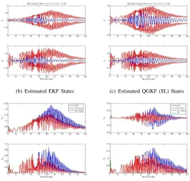
(a) True and Estimated States (b) Estimated EKF States (c) Estimated QGKF (SL) States
(d) Estimated QGKF (DE) States (e) Diagonal Components of State Estima-tion Error Covariance Matrix
(f) Off-Diagonal Components of State Esti-mation Error Covariance Matrix
Fig. 1. Simulation Results for Case1
(a) True and Estimated States (b) Estimated EKF States (c) Estimated QGKF (SL) States
(d) Estimated QGKF (DE) States (e) Diagonal Components of State Estima-tion Error Covariance Matrix
(f) Off-Diagonal Components of State Esti-mation Error Covariance Matrix
The above discussion brings out the fact that for the case of high and low nonlinearity in system dynamics and measurement equations, the QGKF always outperforms the EKF. Finally, we mention that although we have not proved the positive definiteness of updated state covariance matrix in the QGKF, we did not face difficulties associated with such issues.
VI. CONCLUSIONS
In this paper, we have presented a quasi-Gaussian Kalman filter for continuous dynamical systems. We have used the moment evolution equations for stochastic continuous dy-namical systems in order to evaluate the prediction terms involved in the nonlinear filtering recursions. For the inno-vations terms, we have proposed two methods, one based on stochastic linearization and another based on direct eval-uation of the measurement covariance and the state mea-surement cross covariance matrices. We have implemented the filters on a duffing oscillator example and compared the performance to that of an EKF.
It was noted that the complexity of the calculations in-volved in evaluating the prediction and innovations terms are of the same order as that of finding any general higher order moment of a Gaussian random vector, when the nonlinearities are of polynomial type. As such these can be efficiently calculated using Gauss-Hermite quadratures or the Wick formulas. Further, unlike in sigma point filters there is no design criterion for forming the set of sigma points to evaluate the prediction or the innovations terms. In general, higher order moments of the state variable are involved in evaluating the prediction and innovations terms which seems to lead to better performance of the filter. Also, given the dynamics and the measurement equations, the evaluation of these higher order moments can be “hardwired” in order to implement the filter in real time. However, any real time application of this filter would be dictated by the efficiency with which the moment calculations can be accomplished. Hence, there is need for further research into this aspect of the problem.
We also mention that proving the positive definiteness of the updated covariance matrix for a nonlinear system (using any filtering algorithm for that matter) is an open problem in the field of filtering theory. This is also a significant drawback with the proposed filter as it can lead to oscillatory/unstable behavior. However, we did not face such behavior in the example treated in this paper. It is seen from the example that the QGKF performs better than the EKF even for a highly nonlinear system. Thus, the stability properties of the proposed filter could be another direction of further research. Finally, we appreciate the truth that results from any test are difficult to extrapolate, however, testing the new filtering algorithm on a reasonable nonlinear system and providing comparisons to the most obvious competing algorithms does provide compelling evidence and a basis for optimism.
REFERENCES
[1] R. E. Kalman, “A New Approach to Linear Filtering and Prediction Problems”,Trans. ASME Journal of Basic Engineering, pp 35-45, 1960.
[2] H. J. Kushner, “Dynamical Equations for Optimal Nonlinear Fil-ter”’, Journal of Differential Equations, vol. 3, no. 2, 1967, pp. 179-190.
[3] H. J. Kushner, “Nonlinear filtering: The Exact Dynamical Equa-tions satisfied by the Conditional Mode”, IEEE Transactions on Automatic Control, vol. 12, 1967, pp. 262-267.
[4] A. H. Jazwinski, “Stochastic Processes and Filtering Theory”, vol. 64,Mathematics in Science and Engineering, Academic Press, New York, 1970.
[5] R. L. Stratonovich, “Conditional Markov Processes”, Theory of Probability and Its Applications, vol. 5, 1960, pp. 156-178. [6] H. J. Kushner, “Approximations to Optimal Nonlinear Filters”,IEEE
Transactions on Automatic Control, AC-12(5), pp. 546-556, October 1967.
[7] R. P. Wishner, J. A. Tabaczynski, and M. Athans, “A Comparison of Three Nonlinear Filters”,Automatica, vol. 5, pp. 487-496, 1969. [8] L. Schwartz and E. B. Stear, “ A Computational Comparison of Several Nonlinear Filters”, IEEE Transactions on Automatic Control, vol. AC-13, pp. 83-86, 1969.
[9] D. L. Alspach amd H. W. Sorensen, “ Nonlinear Bayesian esti-amtion using Gaussian Sum Approximations”’,IEEE Transactions on Automatic Control, AC-17, pp. 439-448, 1972.
[10] J. R. Fisher, “Optimal Nonlinear Filtering”, inAdvances in Control Systems, C. T. Leondes, ed., Academic Press, New York, pp. 197-300, 1967.
[11] R. Beard, J. Kenney, J. Gunther, J. Lawton and W. Stirling, “Nonlinear Projection Filter Based on Galerkin Approximation”, Journal of Guidance, Control and Dynamics, vol. 22, no. 2, March-April 1999.
[12] S. Challa, Y. Bar-Shalom and V. Krishnamurthy, “Nonlinear Filter-ing via Generalized Edgeworth Series and Gauss-Hermite Quadra-ture”,IEEE Transcations on Signal Processing, vol. 48, no. 6, pp. 1816-1820.
[13] B. D. O. Anderson and J. W. Moore,Optimal Filtering, Prentice-Hall, 1979.
[14] A. Gelb, ed.,Applied Optimal Estimation, MIT Press, 1974. [15] S. Julier, J. Uhlmann and H. Durant-Whyte, “ A New Approach for
the Nonlinear Transformation of Means and Covariances in filters and Estimators”, inIEEE Transactions on Automatic Control, AC-45(3), pp. 477-482, 2000
[16] S. J. Julier and J. K. Uhlmann, “A New Extension of the Kalman Filter to Nonlinear Systems”, inProc. AerosSense: The 11th Int. Symp. on Aerospace/ Defense Sensing, Simulations and Controls, 1997.
[17] S. Julier and J. Uhlmann, “ Unscented Filtering and Nonlinear Estiamtion”,Proceedings of the IEEE, vol. 92, no. 3, pp. 401-422, March 2004.
[18] T. Lefebvre, H. Bruyninckx and J. De Schutter, “ Kalman Filters of Non-Linear Systems: A comparison of Performance”,International journal of Control, vol. 77, no. 7, pp. 639-653, 2004.
[19] T. Lefebvre, H. Bruyninckx and J. De Schutter, “Comment on ‘A New Method for the Nonlinear Transformations of Means and Covariances in Filters and Estimators’ ”, IEEE Transactions on Automatic Control, vol. 47, no. 8, Aug. 2002.
[20] R. Van Der Merwe and E. A. Wan, “The Square Root Kalman Filter for State and Parameter Estimation”, inProceedings of the Inter-national Conference on Acoustic, Speech, and Signal Processing (ICASSP), Hong Kong, April 2003.
[21] K. Ito and K. Xiong, “ Gaussian Filters for Nonlinear Filtering Problems”’,IEEE Transactions on Automatic Control, vol. 45, no. 5, pp. 910-927, May 2000.
[22] H. Risken,The Fokker Planck Equation: Methods of Solution and Applications, vol. 18, Springer Series in Synergetics, Springer-Verlag, Berlin, 1989.
[23] A. Doucet, N. de Freitas and N. Gordon,Sequential Monte-Carlo Methods in Practice, Springer-Verlag, April 2001.
[24] R. C. Nigam, Introduction to Random Vibrations, MIT Press, Cambridge, MA, 1983.