Abstract
The role of money demand in monetary policy is indisputable. This study analyzes the determi-nants of Indonesian money demand. It uses Insukindro-Error Correction Model, based on Keynes-ianand Monetarist theories. It finds that model based on Monetarist theory is preferable. Estima-tion on the chosen model suggests that money demand for real currency is influenced, in the short term, by total wealth, consumer price index, the red letter religious day, monetary crisis, and in the long term, by domestic interest rates, foreign interest rates, consumer price index, and stock price index. In addition, monetary policy using Certificate of Bank Indonesia, does not influence money demand.
Keywords: Money demand, keynesian and monetarist model, insukindro-error correction model
JEL classification numbers: E41, E49
Abstrak
Peran permintaan uang dalam kebijakan moneter tidak diragukan lagi. Studi ini menganalisis faktor-faktor penentu permintaan uang di Indonesia. Alat analisis yang digunakan adalah Insukindro-error correction model, dengan dasar teori Keynesian dan Monetaris. Studi ini menemukan bahwa model berdasarkan teori monetaris adalah model terbaik. Estimasi pada model tersebut menunjukkan bahwa permintaan mata uang riil dipengaruhi, dalam jangka pendek, oleh total kekayaan, indeks harga konsumen, hari libur agama, krisis moneter, dan dalam jangka panjang, oleh tingkat bunga domestik, tingkat bunga luar negeri, indeks harga konsumen, dan indeks harga saham. Studi ini juga menunjukkan bahwa kebijakan moneter, terutama yang menggunakan Sertifikat Bank Indonesia, tidak mempengaruhi permintaan uang.
Keywords: Permintaan uang, model keynesian dan monetarist, insukindro-error correction model
JEL classification numbers: E41, E49
INTRODUCTION
Money demand plays an important role in monetary policy within any economic situation. The literatures on money demand discuss either theoretical or empirical factor on money demand in both developing and developed countries are abundantly found. Meanwhile, it is indisputable that the monetary policy has reached its economics goals. According to Friedman (1968), the monetary policy can be of any contribution to reaching the economic stability through a strong monetary control. Since the
emer-gence of Classical theory on money de-mand, there has been a long discussion of monetary economic analysis on the ques-tion of “what is the most suitable and eligi-ble model to observe money demand haviour among people?” This issue be-comes crucial as different theory chosen by the observer will lead to different form and function of money demand model, resulting in different macroeconomic mechanism and economic policy as the implication (In-sukindro, 1998).
na-tional addina-tional currency money demand is implemented by considering the develop-ment on economic condition aimed at fa-cilitating money endogeneity. The model of currency outside banks (COB) adopting Error correction Model (ECM) two-step Engle Granger approaches the estimation. The ECM model is basically a model con-cept of econometric-time series which ap-pears to adjust the short run equilibrium with long run equilibrium through adjust-ment process. Meanwhile, the variable se-lection for COB equation is ad hoc and it is assumed that the macroeconomic variables such as GDP, inflation, interest rate s, and exchange value influence it. This means that a mistake on determining macroeco-nomic variables will result in an inaccuracy of the estimation on money demand in In-donesia, which in turn, the calculation on money supply in economy will not be accu-rate for the real economic needs.
Studies on theories and empiric on money demand reveals that many variables influence the money demand; however, wealth as one variable has not sufficient attention in any researches in Indonesia. This may happen as the Keynesian money demand analysis, which is a short term analysis, believes that the wealth is con-stant, in that it eventually is erased. Wealth is an important concept stated in Friedman economic analysis, in which Friedman also believes that wealth is consisting of human and non-human wealth. Therefore, this re-search will be directed to the development of money demand variables which are ab-sent from any attention especially in devel-oping countries, in addition to see the rela-tion behaviour among variables.
Next, the attention will be focused on Keynesian and Friedman concept with his wealth variable, and also on the portfo-lio theory of the money demand which is influenced by risk factor together with the result from the money plus other non-monetary assets such as the expected real return of investment. Furthermore, the
re-search is directed to see the effectiveness of the intervention of monetary policy by in-cluding the shock variable, especially the SBI (Certificate of Bank Indonesia) interest rate in affecting the money demand which is perceived as the intermediate target of a monetary policy. Other focus is on testing the model stability to see the stability of the parameters for the models in order to have reliable long term estimation in the mone-tary policy making. Besides the mentioned variables, the writer will also include the non-economic variables such as dummy variable of red -letters public holidays in addition to the dummy variable of mone-tary crisis together with shock variables in I-ECM model (Insukindro-Error Correction Model). The shock variable is the govern-ment-controlled variable, as like the inter-est rate of Certificate of Bank Indonesia. By doing so, one can find out the effective-ness of the intervention on monetary policy which affects the money demand (Yuliadi, 2006).
The goals of the research on the phenomena of currency and chartal money demand are specifically formulated as fol-lows. (a) Analyzing the factors influencing the currency money demand in Indonesia. (b) Analyzing the effectiveness of control-ling money demand by the Certificate of Bank Indonesia. (c) Formulating the model of currency money demand in Indonesia.
positively. Meanwhile, Keynesian theory mentions that the money demand is influ-enced by the motives to keep the money: transaction and precaution motives, which are also influenced positively by an in-come. The speculation motive on the other hand is influenced negatively by the inter-est rates (R). The development of the the-ory is signed by the emergence of Friedman theory stating that the money demand is influenced by a lot of factors such as price (P) which negatively influences, return of obligation (rb), return of stock (re) also negatively influences, wealth (W) posi-tively influences, preferences (u) positively influences.
The portfolio theory, the continua-tion of Friedman theory on the demand for money, mentions that the demand is influ-enced by quite similar factors of Friedman theory, only there has been additional fac-tor such as the expected price (πe) which influences negatively. Meanwhile, the Baumol and Tobin’s theory has different argument in that the money demand is in-fluenced by how much the cost to hold the money which are rate of interest (R) and price (P) which can give a negative influ-ence. Next, Mundell-Fleming theory states that the demand on the real money balance depends negatively on domestic rate of in-terest (R) which is determined by the world rate of interest (R*) and positively influ-ence the income (Y). Islam then offers other theory of money demand stating that money is principally provided for produc-tive sector (transaction). Therefore the ac-tivity such as hoarding money needs to be discouraged. In other words, besides real income and level of inflation, the demand on money is also influenced by tax on inac-tive asset as a negainac-tive influence, total of government expense which is a positive influence, ratio of share between shahibul mal and mudharib in bank which is a nega-tive influence, reserve requirement as the public policy, and objective information of
society in the real condition of economy (Muhammad, 2002).
METHODS
This research will use secondary data dur-ing 1990-2008 which is a monthly data, therefore the number of data (n) is 228. The collected data covers: (a) currency money in million, (b) Gross Domestic Product as a constant price in 2000 in million rupiahs, (c) time deposit interest rate of 1 month in percentage, (d) the rate of interest of 3-month LIBOR in percentage, (e) exchange rate of rupiah against US dollar, (f) cus-tomers price index of 2002, (g) rate of in-terest of 3-month SBI in percentage, (h) Indonesia Composite Index on the closing index, (i) total wealth proxy from primary money and GDP with Friedman formula-tion.
Model Specification
To use the model of I-ECM, the writer conducts an observation on the model specification of the expected money de-mand, both in Keynesian (1) and Monetar-ist models (2) such as:
Model I (Keynesian):
Mdt* = 1.0 + 1.1GDPt + 1.2RD1t + 1.3RLNt + 1.4ERt+ 1.5IHKt
+ 1.6DUMHB1t+ 1.7DUMKt (1) Model II (Monetarist) :
Mdt* = 2.0 + 2.1TWt + 2.2RD1t
+ 2.3RLNt + 2.4IHSGt + 2.5IHKt + 2.6DUMHB1t
+ 2.6DUMKt (2)
as-sumed that the difference appears because of the shock and the late adjustment which follows, therefore, the difference can be found by using the two models (1) and (2) as follows: (Insukindro, 1998)
DE = Mdt* - 3.0 + 3.1GDPt + 3.2RDt
+ 3.3RLNt + 3.4ERt+ 3.5IHKt + 3.6DUMHB1t + 3.7DUMKt (3)
DE = Mdt* - 4.0 + 4.1TWt + 4.2RDt + 4.3RLNt + 4.4IHSGt + 4.5IHKt + 4.6DUMHB1t + 4.7DUMKt (4) The different value is known as disequilib-rium error. And then by modifying the ap-proach that has been developed in Do-mowitz and Elbadawi (1987), the function of the square cost of single period will be as follows:
Ct = µ(MPt – Mt*)2
+ {(1–B) (MPt – jZt)}2 (5)
MPt = Mt – Ut dan Ut = λ(Udt +
(1 - λ) Ust (6)
Substitute the (6) equation to (5) equation leading to:
Ct = µ(Mt – Ut – Mt*)2
+ {(1 – B)( Mt – Ut – jZt)}2 (7) Notes :
C is cost of economic actor
MP is quantity of planned money de-manded in the short term
M* is quantity of the planned money de-manded in the long term
M is real money demanded U is variable shock shock variable
Ud is variable of shock vector that influ-ences the money demand.
Us is variable of shock vector that influ-ences the money
B is t-lag operator
The first component of equation (7) is the cost of imbalances while the second
one is the adjustment cost, µ and are the line vectors that give values to each cost. Zt is the variable vector influencing the amount of money on demand and is per-ceived as linearly influenced by independ-ent variables on model (1) and (2) above. J value mirrors the line vector that gives weight to the element (1-B)Zt. The compo-nent then is included as adjustment cost component as it is seen that the observed system does not exist around the Mt-1 envi-ronment and also because the growth of all variables in the model is constant (Insukin-dro, 1998).
The appearance of money demand variable in short term plan and shock U variables in the equation of (5), (6) and (7) are to cover the possibility of the emer-gence of unanticipated variable from both demand and supply. Next, substitute the Zt as the function of GDPt, RD1t, RLNt, ERt,
IHKt, dumHBt, dumKt (model I) and TWt,
RD1t, RLNt, IHSGt, IHKt, DUMHB1t,
DUMKt (model II), and therefore minimiz-ing the cost function (7) to Mt resulted in:
Mdt = 8.0 + 8.1GDPt+ 8.2RD1t + 8.3RLNt + 8.4ERt + 8.5IHKt + 8.6DUMHB1t + 8.7DUMKt + 8.8GDPt-1 +
8..9RD1t-1 + 8.10RLNt-1 + 8.11 ERt-1 + 8.12IHKt-1 + 8.13Mt-1 + 8.14Ut +
8.15Ut-1 (8)
Mdt = 9.0 + 9.1TWt + 9.2RD1t + 9.3RLNt + 9.4IHSGt + 9.5IHKt + 9.6DUMHB1t + 9.7DUMKt + 9.8TWt-1+ 9.9RD1t-1 + 9.10RLNt-1 + 9.11IHSGt-1 +
9.12IHKt-1 + 9.13Mt-1 + 9.14Ut +
9.15Ut-1 (9)
sta-tionary, If the variables of the model are not stationary then the model cannot be es-timated by using OLS (ordinary least square) method as it will trigger the spuri-ous regression or spurispuri-ous correlation (Thomas, 1997 in Insukindro, 1998). As a solution, the change (d) on level of variable enabling the stationary condition is applied. Therefore, the equation of (8) and (9) should be reparameterized and stated in the form of log-linier and dependent variable with currency real money (CRTL) and real CHARTAL money (GRRL) are included, which results in the following model: Model I (Keynesian)
dlnCTRLt = 10.0 + 10.1 dlnPDBt + 10.2
dRD1t+ 10.3 dRLNt + 10.4 dlnERt + 10.5 dlnIHKt + 10.6 DUMHB1t + 10.7
DUMKt + 10.8 lnBPDBt + 10.9 BRD1t + 10.10 BRLNt + 10.11 lnBERt + 10.12 lnBIHKt + 10.13 ECT + 10.14 dUt + 10.15BUt (10) Model II (Monetarist)
dlnCTRLt = 11.0 + 11.1 dlnTWt + 11.2
dRD1t + 11.3 dRLNt + 11.4 dlnIHKt + 11.5 lndIHSGt + 11.6 DUMHB1t + 11.7 DUMKt + 11.8 lnBTWt + 11.9 BRD1t + 11.10 BRLNt + 11.11 lnBIHKt + 11.12 lnBIHSGt + 11.13
ECT + 11.14 dUt+ 11.15 BUt (11) where
Md is money demand,
CTRL is currency money demand, GRRL is CHARTAL money demand, PDB is national income,
RD1 is domestic rate of interest, RLN is foreign interest rates, IHK is price change,
IHSG is return of real stock, TW is wealth,
DUMHB1 is Dummy variable of Eid Fitr, DUMK is Dummy variable of
eco-nomic crises,
ECT is coeficient of adjustment, U is shock variable,
ER is exchange rate, D is delta,
B is t-lag operator (t -1).
The characteristic of I-ECM model is valid as it meets the condition that the coefficient value of ECT is found 0 < 10.13, 11.13 < 1 positive and statistically must be significant. If it meets the condition, then the I-ECM model can be used as a valid estimation method.
RESULTS DISCUSSION Unit Root Test
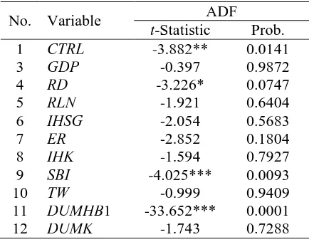
The result of stationary test on Table 1 re-veals that the variables can reach stationary level by testing the unit roots of Aug-mented Dickey-Fuller (ADF). There are 4 variables which are CTRL, RD, SBI and DUMHB1, as the value of ADF statistic absolute is larger than McKinnon statistic absolute on each or the probability is be-low 10%. The data of CTRL reaches sta-tionary on the critical value 5%, RD is in stationary on the critical value 10%, SBI on critical value 1% and DUMHB1 on critical value of 1%. Meanwhile the other variables are not stationer. As some data in the analysis are not stationary on the level or I(0) then the testing for the degree integra-tion.
Table 1: Unit Roots Test on Each Level No. Variable t-Statistic ADF Prob.
1 CTRL -3.882** 0.0141 3 GDP -0.397 0.9872 4 RD -3.226* 0.0747 5 RLN -1.921 0.6404
6 IHSG -2.054 0.5683
7 ER -2.852 0.1804 8 IHK -1.594 0.7927 9 SBI -4.025*** 0.0093 10 TW -0.999 0.9409 11 DUMHB1 -33.652*** 0.0001
12 DUMK -1.743 0.7288
Notes: ***, **, and * represent stationary at 1%, 5%, and 10%, respectively.
Integration Test
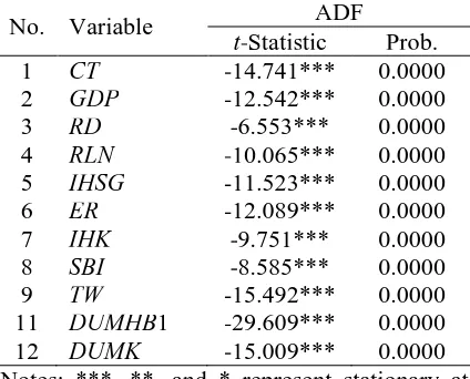
The non stationary data on the test of unit roots is continued with the test on the unit roots of DF on the first difference to finally get the stationary data. If the expected re-sult is not in the stationary situation then the unit root test on the second difference or I(2) is conducted, and etc. The calcula-tion on unit roots of the first difference can be observed on the table 2 below. The table shows that the test of unit roots on the first difference for all variables reached station-ary condition on the first difference on critical value 1%. It occurs as all the lute values of ADF are larger than the abso-lute statistic of McKinnon or the probabil-ity value is lower than 1%. Therefore, if the level of the variables in the analysis has met the stationary level on the first differ-ence, then it needs to undergo a change or delta on the level of variables enabling to reach the stationary condition or null inte-grated or I(0). By that way, the model can be estimated by using Ordinary Least Square (OLS).
Table 2: Result of Unit Root Test on the First Difference Equation Model No. Variable t-Statistic ADF Prob. 1 CT -14.741*** 0.0000
2 GDP -12.542*** 0.0000
3 RD -6.553*** 0.0000
4 RLN -10.065*** 0.0000
5 IHSG -11.523*** 0.0000
6 ER -12.089*** 0.0000
7 IHK -9.751*** 0.0000
8 SBI -8.585*** 0.0000
9 TW -15.492*** 0.0000
11 DUMHB1 -29.609*** 0.0000
12 DUMK -15.009*** 0.0000
Notes: ***, **, and * represent stationary at 1%, 5%, and 10%, respectively.
Source: Data estimation.
Cointegration Test
The first step to do the cointegration test is finding the residual data (et) on the
regres-sion model used in the analysis. The co-integrated test is using the basic model of money demand as in the model I and II previously. Having been found, the residual data is tested by using the root unit test in order to find out the stationary. Supposed the residual of the equation is stationary I (0) the variables then are cointegrated which means they have long term relation. Table 3 shows both the statistics and prob-ability values of the residual co-integration from each model. From the table, the result of the estimation on the model of Aug-mented Dickey-Fuller shows that model I CTRL and model II CTRL have absolute values of ADF t-statistics which is larger than Mckinnon absolute statistic value or it also means that the probability is lower than 1 %, which means that there is an in-dication that the residual variable of each model for the level data does not contain root unit, or in other words, the residual variable is already in stationary condition I(0) on critical value 1%. It can be con-cluded then that the co-integration occurs among all variables involved in the model of the money demand. It means that in the long term, the balance or stability amongst the observed variables occurs.
Table 3: Cointegrated Test on the Money Demand Model
No. Model t-Statistic Probability ADF 1 Model I
CTRL -5.485*** 0.0000 3 Model II
CTRL -2.871*** 0.0042 Notes: ***, **, and * represent stationary at 1%, 5%, and 10%, respectively.
Source: Data estimation.
The Validity of Keynesian Currency Money Demand
heteroscedasticity test, it is found that the CTRL Model I does not contain heterosce-dasticity as the Obs*R2 value or 2 value of calculation model 35.075 is smaller than 2 critical value (on = 5 % and df = 28) for 41,337 or by considering the chi-square probability value for 0.168 larger than 5%. Next on the linearity test, the model I CRTL with Ramsey RESET test shows that the calculated F is 10,246 larger than critical F on = 5 % with df (1, 208) for 3,89 or by considering the statistic F probability 0.0016 lower than 5% so that the model signifi-cantly refused H0 stating that the linear-shaped model means the non-linear one.
The estimation of Model 1 of real currency demand (Model 1 CRTL) as in Ta-ble 4 can be found by using OLS as all the key variables in I-ECM have the stationary data. The calculation using the facility of Eviews software package finds that the
posi-tive-marked ECT coefficient and significant means that it meets the expectancy and sup-ports the result of the co-integration test which tells that LNCTRL, LNGDP, RD1, RLN, LNER, LNIHK, DUMHB1 and DUMK variables are co-integrated or they have the long-term balance.
The elasticity of each variable shows that in the short term, real currency demand is influenced by the real income (GDP) exchange rate (ER) and variable of public holiday (DUMHB1) significantly. Only then, the GDP variables have nega-tive elasticity which does not meet the ex-pectation of the theories where GDP vari-able has positive mark. However, the be-haviour of the short term elasticity is dif-ferent from that of a long term where GDP variable has positive mark. Then for other variables such as RD, RLN, ER, IHK, they have significant influence in the long term. Table 4: Estimation Result on Keynesian Demand on Currency
No. Variable Coefficient Model I CTRL t-statistic
1 D(LNGDP) -1.168770 -2.895010***
2 D(RD1) 0.000582 0.336216 3 D(RLN) 0.018267 1.568479 4 D(LNER) 0.108823 2.387914**
5 D(LNIHK) -0.385718 -1.288357
6 DUMHB1 0.065970 8.323079***
7 DUMK -0.030778 -1.282303
8 LNGDP(-1) 0.092357 1.712855*
9 RD1(-1) -0.510696 -10.12094*** 10 RLN(-1) -0.506411 -10.09924*** 11 LNER(-1) -0.378403 -7.925595***
12 LNIHK(-1) -0.558952 -8.468188***
13 ECT 0.509082 10.11144*** 14 D(SBI) 0.001773 1.435725 15 SBI(-1) -0.000696 -0.580261
16 CONSTANT -4.610849 -5.862106***
R2 0.501059 Adjusted R2 0.465589 S.E. of regression 0.043254 Akaike info criterion -3.375577 Schwarz criterion -3.134171
F-statistic 14.12635*** Durbin-Watson stat 2.139931
N 227
Validity of Monetarist Currency Money Demand
As in the model I above, prior to the analy-sis of the estimated model, the model test-ing is conducted. Based on the White Het-eroskedasticity test calculation for testing the heterocedasticity on the Monetarist model, it is found that the model II CRTL contains the heteroskedacity. The White Heteroscedasticity test calculation on the model II CTRL 2 value of the model calcu-lation 74,195 bigger 2 value, critical (on = 5 % with df = 28) as much 41,337 or by seeing the probability score of chi-square 0,000005 lower than 5 % which means that it doesn’t pass the heteroscedasticity. Next, for linearity test, the model II CTRL with Ramsey RESET test found that calculated F-statistic is 0.041 lower than F-critical when = 5 % with df (1;208) 3.89 or by considering the probability of statistic F = 0.839 larger than 5% so that the model does not significantly accept H0 stating that the model is in linear shape.
The estimation model II CTRL in Table 5 has stationary variable that the model can be estimated using ordinary least squares. The computational result says that ECT coefficient marked positive and sig-nificant means it fits the expectation and supports co-integrated computational result which shows LNCTRL. LNGDP, RD1, RLN, LNER, LNIHK, DUMHB and DUMK variable has cointegrated or had a long-term balance relation. Furthermore, when viewed from the elasticity of each variable, it turns out that real currency money de-mand in the long run is apparently influ-enced by total wealth variable (TWV), hol i-day dummy (HD1), crisis dummy (CD). These have significant and positive influ-ence; while consumer price index (CPI) has significant and negative influence, and other variables have insignificant influence over real currency money demand. Never-theless, when viewed from the long-run elasticity, nearly all variables (RD1, RLN, IHK, IHSG) show significant influence.
Table 5: Estimation Result of Monetarist Currency Money Demand
No. Variable Coefficient Model II CTRL t-statistic
1 D(LNTW) 1.254340 12.36541***
2 D(RD1) 0.000435 0.275241
3 D(RLN) 0.010983 1.001083
4 D(LNIHK) -0.416093 -1.676073*
5 D(LNIHSG) -0.015180 -0.485971
6 DUMHB1 0.029197 3.716480***
7 DUMK 0.032622 1.738613*
8 LNTW(-1) -0.031392 -0.672944
9 RD1(-1) -0.155842 -4.07462***
10 RLN(-1) -0.154652 -4.328383***
11 LNIHK(-1) -0.196108 -3.829583***
12 LNIHSG(-1) -0.161062 -3.879101***
13 ECT 0.154961 4.315017***
14 D(SBI) -0.000285 -0.260321
15 SBI(-1) -0.000911 -0.809120
16 CONSTANT -0.323990 -0.856022
R2 0.576130
Adjusted R2 0.545997
S.E. of regression 0.039867
Akaike info criterion -3.538638
Schwarz criterion -3.297232
F-statistic 19.11959***
Durbin-Watson stat 2.417209
N 227
Empirical Model Selection
Economy theories have widely investigated balance relation and covered economy variables within a theoretical economy model. In the theory, however, the relation form amongst economy variables is not discussed specifically and various variables in empirical economy model are not sug-gested. Thus, selecting empirical model has become important for obtaining a good model (Insukindro and Aliman, 1999).
The model selection in this research makes use of non-nested test due to inde-pendent specification of the models – a model is separated from other models. Put in another way, both models have same de-pendent (Y) and different independent vari-ables. This model is called non-nested model as model 1 is not a part of model 2 and conversely model 2 is not a part of model 1. The selection of non-tested model in this research uses some criterion, as fol-low: (a) goodness of fit criterion – the coef-ficient of determination R2 and adjusted coefficient of determination R2 , (b) Akaike’s Information Criterion (AIC), and (c) Schwarz’s Information Criterion (SIC).
The econometrics experts have de-veloped a statistical test for selecting a good model - in which two models have same dependent variables by either coeffi-cient of determination criterion (R2) or ad-justed coefficient of determination R2 . The estimation model selected is the one which has R2 or R2 value higher than other models. Based on goodness of fit criterion, the computation for coefficient of determi-nation R2 and adjusted coefficient of deter-mination R2 (view Table 4 and 5), known that the estimation model of real currency money demand by monetarist model, has R2= 0.576 and R2 = 0.546. It is better than Keynesian model, which has R2= 0.501 and
2
R = 0.466. Thus, CTRL estimation model by monetarist has performed better than Keynesian.
The Estimation Model of Monetarist Currency Money Demand
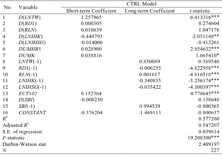
By the analysis of the two criterions of se-lecting model by goodness of fit, AIC and SIC, it can be concluded that real currency money demand by monetarist model has performed better than Keneysian. The es-timation model of monetarist currency money demand (Table 6) has been amelio-rated with output Newey-West HAC Stan-dard Errors & Covariance that the the re-covery of heteroscedasticity has been ex-amined. From the table, it can be explained that I-ECM model constructed as expected – the coefficient value of ECT is positive and significant. This means the estimation model of money demand is valid, if the co-efficient value of error correction term is not equivalent to zero and signifi-cant. So, in other words, I-ECM model works and can be used for estimating the factors that influence money demand in Indonesia during the research period. The result also indicates that the model specifi-cation is valid and accordance with the re-sult obtained in cointegration regression as in previous discussion. The estimation re-sult has coefficient of adjustment value
14.15 = 0.152364. It means that approxi-mately 15.23% the discrepancy between the actual and expected LNCTRLt will be eliminated or omitted within a month.
Table 6: EstimationResult of the Monetarist Currency Money Demand Model
No. Variable Short-term Coefficient Long-term Coefficient CTRL Model t-statistic 1 D(LNTW) 1.257965 6.413316***
2 D(RD1) 0.000305 0.274604
3 D(RLN) 0.010639 1.047176
4 D(LNIHK) -0.449793 -2.051148**
5 D(LNIHSG) -0.014006 -0.412261
6 DUMHB1 0.028900 2.854632***
7 DUMK 0.038816 1.665410*
8 LNTW(-1) 0.850089 -0.389546
9 RD1(-1) -0.006255 -4.822958***
10 RLN(-1) 0.001017 -4.816518***
11 LNIHK(-1) -0.340835 -3.256174***
12 LNIHSG(-1) -0.035422 -4.300397***
13 ECT102 0.152364 4.778645***
14 D(SBI) -0.000230 -0.138648
15 SBI(-1) 0.994539 -0.800365
16 CONSTANT -0.376204 -1.469113 -0.800637
R2 0.577260
Adjusted R2 0.547207
S.E. of regression 0.039814
F-statistic 19.208300***
Durbin-Watson stat 2.409197
N 227
Notes: ***, **, and * represent significant at 1%, 5%, and 10%, respectively. I-ECM Model of long-term coefficient is formulated as ( i + 12.13)/ 12.13.
Source: Data estimation.
Short-Term Analysis on Monetarist Currency Money Demand
The result of short-term currency money demand analysis constitutes four significant variables which have influence; total wealth variable (TWV), consumer price in-dex (CPI), holiday dummy (HD1), mone-tary crisis dummy (MCD). Wealth variable and holiday dummy statistically are signifi-cant with = 1 %, consumer price index variable is significant on = 5 %, crisis dummy variable (MCD) is significant on = 10 %. Wealth variable has the coefficient 1.25797, which means if total wealth in-creases 1%, real currency money demand increases 1.25797%. This finding is in line with Daquila and Fatt (1993), and Martin and Winder (1998) that shows the influence of wealth towards money demand is posi-tive and significant. For consumer price index variable (CPI), it has significant
in-fluence with 0.44079 coefficient. This means total wealth increases 1%, real cur-rency money demand declines 0.44079%. This is in line with studies conducted by Boediono (1985), Daquila and Fatt (1993), Sugiyanto (1995), Neil and Sharma (1998), Hayo (2000).
period with 0.0388 coefficient, which means it is higher in and post crisis period than that pre crisis period.
For other variables RD1, RLN, IHK, IHSG, they do not influence significantly real currency money demand in the short term. For policy variable, in the short term, it does not either. This condition indicates variables established in the short term give less influence over the change of real cur-rency money demand in Indonesia. By this analysis, it can be explained also that short-term currency money demand is not elastic to interest rates, both domestic and foreign interest rates. This is empirically in line with the economic theory indicating that money demand in the short term is allo-cated for transactions and uncertainties. This is accordance with Insukindro’s find-ing (1998), that short-term money demand is more allocated for transactions and un-certainties, not for speculations.
Long Term Analysis of Monetarist Cur-rency Money Demand
Long-term analysis on factors that influ-ence real currency money demand suggests that domestic interest rates variable has significant influence on towards real currency money demand. Its long-term coefficient is -0.006255, which means if interest rates rise to 1%, the demand for currency money will fall 0.006255%. For foreign interest rates variable, it has signifi-cant influence on towards real cur-rency money demand with long-term coef-ficient 0.001017. It means if foreign inter-est rates rise to 1%, the demand for cur-rency money will rise to 0.001017%. Then, for price level variable or consumer price index (CPI), it has significant influence on = 1 % towards real currency money de-mand with long-term coefficient -0.340835. This means if consumer price index rises to 1%, the demand for currency money will fall to 0.340835%. The influence of com-posite stock price index as a proxy from return of the stock turns out to affect
sig-nificantly real currency money demand with and the longterm coefficient -0.03542. This means if composite stock price index rises to 1%, it will decrease the demand for currency money 0.03542%.
The findings above on the influence of domestic interest rates variable, con-sumer price index, composite stock price index towards money demand are in line with the theories. Domestic interest rates with negative influence is in accordance with the studies conducted by Boediono (1985), Fair (1987), Insukindro (1993), Daquila and Fatt (1993), Honohan (1994), Ericsonand Sharma (1998), Obben (1998), Eitrheim (1998), Xu (1998), Skrabic and Tomic (2009), Nautz and Ulrike (2010), Abdullah et al. (2010), Odularu and Okun-rinbuye (2009), Valadkhani (2008), Singh andManoj(2009), Achsani(2010), Hamori (2008). Consumer price index (CPI) with negative influence is in accordance with studies by Boediono (1985), Widjanarko (1989), Daquila and Fatt (1993), Sugiyanto (1995), Neil and Sharma, (1998), Bernd (2000). Composite stock price index with negative influence over money demand in Indonesia is in line with Sugiyanto’s study (1995).
Nevertheless, it turns out to give positive and significant influence for for-eign interest rates variable. This is also as investigated by Boediono (1985), Sugi-yanto (1995), Hueng (1999), Elyas and Zadeh (2006), Fair (1987), Daquila and Fatt (1993), Eitrheim (1998), and Abdullah et al. (2010). For policy analysis variable – the influence of monetary policy interven-tion, however, it influences less effectively real currency money in Indonesia. It is proven either in the long term or short term.
CONCLUSION
money (Monetarist) in the short-run was positively influenced by total wealth, nega-tively influenced by consumer index price variable, positively influenced by holiday dummy and positively influenced by crisis dummy. Thus, the demand for currency money was not elastic to interest rates, but to wealth. Consumer price index indicated the demand for currency money in the short- run was allocated for transactions and uncertainties.
Real currency money demand in the long-run was negatively influenced by do-mestic interest rates, positively influenced by foreign interest rates variable, nega-tively influenced by consumer price index, and negatively influenced by composite stock price index. This finding indicated that the demand for real currency money in the long run was allocated for transactions as well as speculations.
In the long-run analysis, the effect of foreign interest rates, either towards real currency money demand, had positive in-fluence, which did not suit the theory. It could be concluded that in the long run, if foreign interest rates rose, the demand for money would rise as well. It was because
people shift money abroad. This condition reasserted that it was not only domestic in-terest rates which affect money demand for speculation purpose, but also foreign inter-est rates. It suited Mundell-Fleming theory stating that Indonesia operated an an open economy.
It could be concluded as well that there was a behavioural difference of cur-rency money demand between holiday and non-holiday month, such as Lebaran and Christmas. Then, for monetary crisis dummy variable, there was apparently a behavioural difference of currency money demand pre and during or post monetary crisis.
From the effect of monetary opera-tion conducted by Bank Indonesia, espe-cially in relation to Bank Indonesia Certifi-cate interest rates, it could be concluded that it had ineffective influence in the short and long-run. This finding indicated that the policy, especially Bank Indonesia Cer-tificate was less able to influence the amount of money supply (currency money), with the economy assumption of equilibrium in money market.
REFERENCES
Abdullah, H., J. Ali, and H. Matahir (2010), “Re-Examining the Demand for Money in Asean-5 Country,” Asian Social Science, 6(7), 146-155.
Achsani, N.A. (2010), “Stability of Money Demand in an Emerging Market Economy: An Error Correction and ARDL Model for Indonesia,” Research Journal of Interna-tional Studies, 13, 83-91.
Boediono (1985), “Demand for Money in Indonesia 1975-1984,” Bulletin of Indonesian Economic Studies, 21(2), 74-94.
Daquila, T.C. and A.P.K. Fatt (1993), “Demand for Money in Singapura Rivisited,” Asian Ekonomic Journal, 7(21), 181-195.
Domowitz, I. and L. Elbadawi (1987), “An Error-Correction Approach to Money Demand: The Case of the Sudan,” Journal of Development Economics, 26, 257-275.
Elyas, A. and A.H.M. Zadeh (2006), “Selection of the Scale Measure in Narrow Money Demand: The Cases of Japan and Germany,” Quarterly Journal of Business and Economics, 45(1), 115-135.
Fair, R.C. (1987), “International Evidence on the Demand for Money,” Review of Econom-ics and StatistEconom-ics, 69(3), 473-480.
Friedman, M. (1968), ”The Role of Monetary Policy,” American Economic Review, LVIII(1), 1-17.
Hayo, B. (2000), “The Demand for Money in Austria,” Empirical Economics, 25(4), 581-603.
Hamori, S. (2008), “Empirical Analysis of the Money Demand Function in Sub-Saharan Africa,” Economics Bulletin, 15(4), 1-15.
Hanohan, P. (1994), “Inflation and the Demand for Money in Developing Countries,” Word Development, 22(2), 215-223.
Insukindro (1998), “Pendekatan Stok Penyangga Permintaan Uang: Tinjauan Teoritis dan Sebuah Studi Empirik di Indonesia,” Ekonomi dan Keuangan Indonesia, XLVI(4), 451-471.
Insukindro and Aliman (1999), “Pemilihan dan Bentuk Fungsi Model Empirik: Studi Ka-sus Permintaan Uang Kartal Riil di Indonesia,” Jurnal Ekonomi dan Bisnis Indone-sia, 14, 49-61.
Martin, F.M.G. and C.C.A. Winder (1998), “Wealth and Demand for Money in European Union,” Empirical Economics, 23, 507-524.
Muhammad (2002), Kebijakan Fiskal dan Moneter dalam Ekononomi Islam, Edisi Per-tama, Salemba Empat, Jakarta.
Nautz, D. and U. Rondorf (2010), “The (In) stability of Money Demand in the Euro Area: Lessons from a Cross-Country Analysis,” Sender Freies Berlin (SFB) 649 Discus-sion Paper, No. 2010-023.
Neil, E.R, and A. Sunil (1998), “Broad Money Demand and Financial Liberalization in Greece,” Empirical Economics, 23, 417-436.
Obben, J. (1998), “The Demand for Money in Brunei,” Asian Economic Journal, 12(2), 109-121.
Odularu, G.O. and O.A. Okunrinbuye (2009), “Modeling the Impact of Financial Innova-tion on the Demand for Money in Nigeria,” African Journal of Business Manage-ment, 3(2), 39-51.
Singh, P. and M.K. Pandey (2009), “Structural Break, Stability and Demand for Money in India,” ASARS Working Paper No. 7.
Skrabic, B. and N. Tomic, (2009), “Evidence of the Long-run Equilibrium between Money Demand Determinants in Croatia,” World Academy of Science, Engineering and Technology Working Paper No. 49.
Valadkhani, A. (2008), “Long and Short-run Determinants of the Demand for Money in the Asian Pasific Country: An Empirical Panel Investigation,” Annals of Economics and Finance, 9(1), 77-90.
Xu, Y. (1998), “Money Demand in China: A Disaggregate Approach,” Journal of Com-parative Economics, 26, 544-564.