1
CHAPTER 1
INTRODUCTION
This chapter is explaining the background of this research, which is determining I-Trolley fleet sizing in a production floor in order to change manual material handling. The problem formulation, objectives, scope, and limitation of this research are also defined as well in this chapter.
1.1. Background
Currently, manufacturing company of this research subject, which is hard drive manufacturer in Thailand, has to face tight competition with many competitors. Company try to have lower price for their products compared to another competitor but still maintain or even higher profit level. The ultimate way to reach the objective is lower the cost to perform an enterprise in form of manufacturing and administration activity.
To respond company objectives, each department responsible to support in their work area. One of department in company, Industrial Engineering Department, is responsible for production activity and make sure that the activity is effective and efficient as possible. In another word, Industrial Engineering Department objectives is to reduce cost in production activity without any reduction on quality, capacity, and reliability. Lean principle becomes one of guideline that can be implemented in the production to achieve the objective. The basic of lean principle is to detect any waste occurred and eliminating waste to have lower manufacturing cost without sacrificing product quality because waste is actually a non-value added activity in production. Waste can be in form of over processing, inventory, transportation, over production, rework, motion, and waiting (Marchwinski & Shook, 2003)
2
AGV is the most popular because one of the reason is AGV can transport almost all type of material to support manufacturing process (Lin et al., 2006). AGV is chose over transportation using man power due to many advantages, such as flexibility, space utilization, productivity, safety, and adaptability with other automated systems (Shneor et al., 2006). Electronic goods manufacturing, in example hard drives manufacturing, also one of well-known example of industry that use AGV in their operations (Gosavi & Grasman, 2009). AGV is known for the best solution of automated material handling in Flexible Manufacturing System (FMS) due to flexibility of AGV route (Leite et al., 2015). The production system in hard drive manufacturer, which is become research subject, can be classified as flow shop. Therefore the concept of AGV is not suitable due to redundancy of the main advantage. Flow shop production system route is fixed from one stations to another stations and all products have same process flow . Instead of using AGV, the manufacturer try to use I-Trolley concept. Currently to support manufacturing activity, company still use manual transportation handling which requires many operators to do the transportation activity. In this project, Industrial Engineering Department is collaborating with Production Engineering Department and Industrial Engineering Department is responsible in calculating the amount of I-Trolley needed to support manufacturing activity and operator reduction to calculate profitability analysis.
I-Trolley principle is actually the same as AGV in term of driverless material handling (Fazlollahtabar & Saidi-Mehrabad, 2015) and consists of many parts, such as: DC Motors, sensors to ensure the safety, wireless communication, and energy sources in form of rechargeable battery (Zajac et al., 2013). The difference between them, I-Trolley is simplification of AGV which are not fully automated and not flexible as AGV system. I-Trolley only has two stop points, one is considered as start point and another is considered as end point. Term usage of start and end point is based on material flow in production. Start point is stop point to load material that ready to be processed to the next station and end point is stop point to unload material in the arrival station.
3
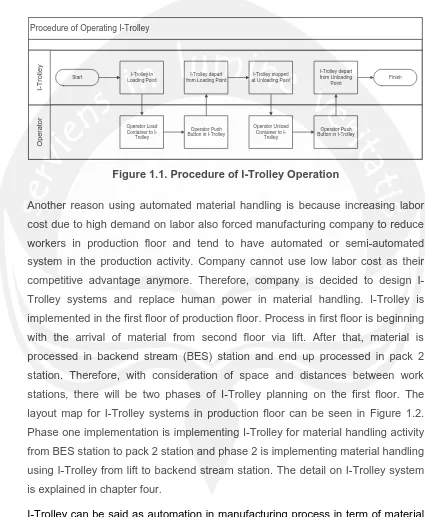
The calculation of transportation times and distances is explained in chapter four. Another consideration of using I-Trolley rather than AGV is because cheaper investment. Cheaper investment is caused by not all features in AGV used in I-Trolley system. The procedure of operator to operate I-I-Trolley can be seen in Figure 1.1.
Procedure of Operating I-Trolley
Operator
I-Trolley
Start Loading PointI-Trolley in
Operator Load Container to
I-Trolley
Operator Push Button in I-Trolley I-Trolley depart from Loading Point
I-Trolley stopped at Unloading Point
Operator Unload Container to
I-Trolley
Operator Push Button in I-Trolley I-Trolley depart from Unloading
Point
Finish
Figure 1.1. Procedure of I-Trolley Operation
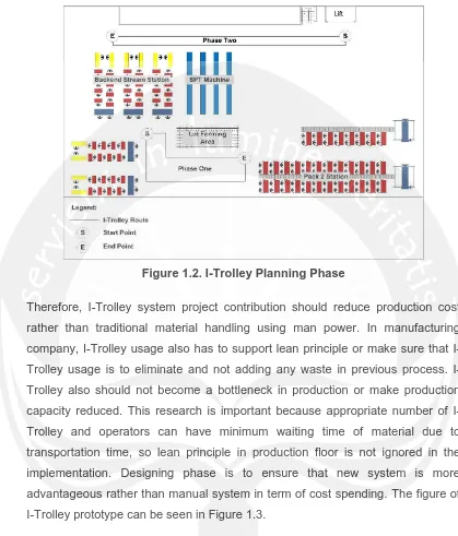
Another reason using automated material handling is because increasing labor cost due to high demand on labor also forced manufacturing company to reduce workers in production floor and tend to have automated or semi-automated system in the production activity. Company cannot use low labor cost as their competitive advantage anymore. Therefore, company is decided to design I-Trolley systems and replace human power in material handling. I-I-Trolley is implemented in the first floor of production floor. Process in first floor is beginning with the arrival of material from second floor via lift. After that, material is processed in backend stream (BES) station and end up processed in pack 2 station. Therefore, with consideration of space and distances between work stations, there will be two phases of I-Trolley planning on the first floor. The layout map for I-Trolley systems in production floor can be seen in Figure 1.2. Phase one implementation is implementing I-Trolley for material handling activity from BES station to pack 2 station and phase 2 is implementing material handling using I-Trolley from lift to backend stream station. The detail on I-Trolley system is explained in chapter four.
4
Figure 1.2. I-Trolley Planning Phase
5
Figure 1.3. I-Trolley Prototype
1.2. Problem Formulation
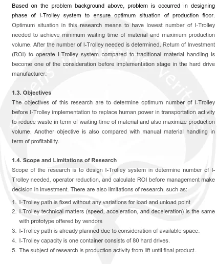
Based on the problem background above, problem is occurred in designing phase of I-Trolley system to ensure optimum situation of production floor. Optimum situation in this research means to have lowest number of I-Trolley needed to achieve minimum waiting time of material and maximum production volume. After the number of I-Trolley needed is determined, Return of Investment (ROI) to operate I-Trolley system compared to traditional material handling is become one of the consideration before implementation stage in the hard drive manufacturer.
1.3. Objectives
The objectives of this research are to determine optimum number of I-Trolley before I-Trolley implementation to replace human power in transportation activity to reduce waste in term of waiting time of material and also maximize production volume. Another objective is also compared with manual material handling in term of profitability.
1.4. Scope and Limitations of Research
Scope of the research is to design Trolley system in determine number of I-Trolley needed, operator reduction, and calculate ROI before management make decision in investment. There are also limitations of research, such as:
1. I-Trolley path is fixed without any variations for load and unload point
2. I-Trolley technical matters (speed, acceleration, and deceleration) is the same with prototype offered by vendors
3. I-Trolley path is already planned due to consideration of available space. 4. I-Trolley capacity is one container consists of 80 hard drives.
6
CHAPTER 2
LITERATURE REVIEW AND THEORITICAL BACKGROUND
This chapter presents some previous researches and theoretical background in automated material handling system, fleet sizing, and economic profitability. Simulation approach and time study which are very useful for this research are also explained in this chapter. Finally, this research contributions over some previous researches are being explained in the last section
2.1. Automated Material Handling System
Groover (2007) give a rough guide in selection of material handling equpiment based on flow rate and distance moved and also based on layout types. Automated material handling system is suitable when flow rate high or/and distance moved low. Rough guide of material handling selection according to Groover (2007) can be seen in Figure 2.1.
Figure 2.1. Material Handling Equipment Based on Flow Rate and Distance
Moved (Groover, 2007)
Type of material handling based on layout type can be divided into three type, fixed-position, process, and product layout type. Fixed position usually related with large product size like airplane manufacturing which has low production rate. Material handling that suitable for fixed position layout type can be cranes or hoists. Another layout type is process layout type which has characteristic in product variability and low production rates. Material handling equipment that suitable for process layout is hand trucks or AGV which have high flexibility in their routing. Last layout types is product layout which has limited product variability and high production rate. Conveyor or powered truck is suitable for
High Conveyors Conveyors, AGV trains Low Manual handling Powered trucks,
Unit load AGV
Short Long
Quantities of
Material Flow
Distance
7
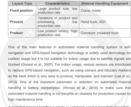
product layout type. Summary of material handling equipment based on layout types can be seen in Table 2.1.
Table 2.1. Material Handling Equipment Based on Layout Type (Groover,
2007)
Layout Type Characteristics Material Handling Equipment
Fixed position Large product size, low
production rate Crane, hoists
Process
Variations in product and
processing, low
production rate
Hand truck, AGV
Product Low product variety, high
production rate Conveyor, powered truck
One of the main features in automated material handling system is self-navigation and GPS-based self-navigation technology is widely used technology for outdoor usage but it is not suitable for indoor usage due to satellite signals are blocked (Grewal et al., 2007). For indoor usage, various sensors are introduced to replace GPS-based navigation, such as using camera and fiduciary markers as the track which is very easy to produce, manipulate, and maintain (Lee et al., 2013). One of the important parameter in selection on automated material handling is battery consumption (Ahmad et al., 2014) to make sure that automated material handling is not become an obstacle for production caused by high maintenance time.
Automated material handling systems is commonly used in manufacturing plants, warehouses, distribution center, and trans-shipment terminals (Rinkacs et al., 2014). The purpose of automated material handling is to connect two stations that cannot be combined due to area constraint and space availability to reduce headcounts in production floor.
2.2. Fleet Sizing
8
material handling. In the beginning research, fleet sizing problems can be similar with queuing theory where fleet is treat as server in queuing theory (Parikh, 1977). Parikh (1977) gave adjustment in queuing model that has same behavior based on inter-arrival time. Situation on his research was automated material handling in flow shop with closed loop route and the objectives is to minimize waiting time of material. The research was continued by Papier and Thonemann (2008) to compared between queueing models and time-space models which is queuing models is more suitable for long term decision making, such as planning fleet sizes over the next years and time-space models is appropriate model to plan allocation for each fleet.
Too little fleet cannot satisfy the requirement, but too many fleet would be increase vehicle cost and traffic intensity (Chang et al., 2014). Chang et al. (2014) used simulation-based framework to find optimum fleet size under multi objective because one of the advantages of using simulation is user can treat some processes as a black box. Chang et al. (2014) use simulation due to complexity in automated material handling route. Another research found that analytical approach is found to be the best solution to determine minimum fleet size under time-window constraint (Vis et al., 2005)
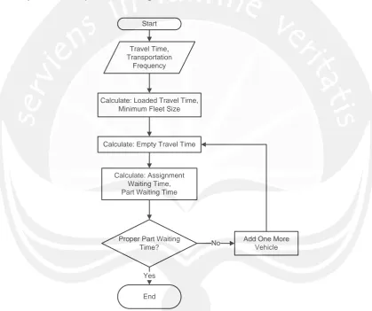
Koo et al., (2004) done some research in fleet sizing for multiple pickup and delivery point with consideration of additional rules of nearest vehicle selection rule. Koo also shows the overall fleet sizing procedure which is shown in Figure 2.2.
To determine minimum fleet size, total vehicle travel time is divided by the length of available time of vehicle (Koo et al., 2004). Automated material handling design for closed loop flowshop already researched by Hall et al., (2001) and fleet sizing was based on minimum cycle time of processes that will not reduced anymore if one material handling was added.
9
2.3. Flow Shop and Queuing Model
Hard disk manufacturers can be classify as flow shop which has characteristic on limited product variability and high production rate. Buzacott & Shanthikumar (1993) breakdown flow shop into certain categories based on characteristic in flow shop. There are two categories based on operator policy in processing item, paced and unpaced lines. Paced lines is condition when cycle time of operator in every work center is fixed. Therefore, it is possible that operator not finish the task given. On the contrary, unpaced lines is condition when there is no limited cycle time of operator in doing their task.
Start
Travel Time, Transportation
Frequency
Calculate: Loaded Travel Time, Minimum Fleet Size
Calculate: Empty Travel Time
Calculate: Assignment Waiting Time, Part Waiting Time
Proper Part Waiting Time?
Add One More Vehicle No
End Yes
Figure 2.2. Overall Fleet Sizing Procedure (Koo et al., 2004)
10
transfer line. Therefore, it can be modelled by an open tandem queueing network. Buzacott and Shanthikumar (1993) also explained when inter-arrival time is poisson distribution and processing time in each server is exponential distribution, it can be solved using queuing model M/M/c. If inter-arrival time is not poisson distribution and/or processing time is not exponential distribution, it can be solved using queuing model G/G/c. Allen-Cunneen aproximation usually gives good approximation for G/G/c system, but unfortunately extensive testing by Tanner give conclusion that the result of approximation are within 10% of true values (Winston & Goldberg, 2004).
Taha (1997) explained about notation in queuing network with general notation a/b/c:d/e/f where a and b are respectively represent of arrival time and service time, c is represent number of server, d is represent queue discipline, e and f are respectively represent of maximum number in system and size of calling source which is infinite or finite. Notation to represent arrival and service time are:
a. M = Markovian (Poisson) arrival or service time which is equivalently with exponential inter-arrival time or service time
b. D = Constant (Deterministic) time
c. Ek = Erlang or gamma distribution of time
d. GI = General (generic) distribution of inter-arrival time e. G = General (generic) distribution of service time
Taha (1997) also explained when queuing model arrival and departure time is not following Poisson distribution, the model will be very complex and it is advisable to use simulation approach.
2.4. Simulation Approach
Winston & Goldberg (2004) defined simulation as a method or tool to depict the operation of a real world system as it evolves over time. System is a collection of entities that act and interact toward the accomplishment of some logical end (Schmidt & Taylor, 1970). Taha (1997) divided two type of simulation model, which are static and dynamic.
a. Static: Representation of a system at a particular point in time b. Dynamic: Representation of system as it evolves over time
11
framework on simulation study, which is shown in Figure 2.3. However, it is not mandatory to use the same framework caused by overlap between some of the stages.There are a lot of simulation software. Kelton et al. (2006) gave information needed such as features and capabilities in using ARENA Simulation software.
Start
Collect data and develop a model
Computerize the model
Verified?
Validated Yes
Yes
Design the experiment
Perform simulation runs
Analyze output data
Simulation Complete?
Yes
Document and implement runs
No
No
No
Finish
12
Kelton et al. (2006) gave framework on analyzing simulation result based on time frame of simulation. There are two time frame of simulations, which are terminating and steady state. Problem occurred in terminating simulation when to determine number of replications. Approximation in determining number of replication can be seen in Equation 2.1.
n ≅z1-α/2 2 s2
h2
(2.1)
Where:
n = Number of replications z = Z-Value
α = Confidence interval
s = Sample standard deviation h = Half-width
Another easier approximation but slightly different can be seen in Equation 2.2.
n ≅n0h0 2
h2
(2.2)
Where:
n0 = Initial number of replications
h0 = Initial half-width
The approximation formula on replication number needed can be defined as same as central limit theory, which is stated that it is fairly good enough if n is large (Kelton et al., 2006). Another stage to be considered in simulation is verification and validation stage. Kelton et al. (2006) gave definition on verification and validation. Verification stage in simulation software is to detect any error in model or ensure simulation behaves as intended. Validation is defined as activity to ensure that the simulation behaves the same as the real situation. There should be one or more parameter that can be compared between real situation and simulation model.
2.5. Statistical Analysis
13
Therefore, statistical analysis is useful to prove the any significance difference between scenarios. There are various tools to prove any significance difference between samples, such as z-test or t-test if there are only two samples involve. The tools in statistical analysis to prove any significance difference between samples if there are more than two samples involve is Analysis of Variance (ANOVA) (Bluman, 2012). Bluman (2012) divide ANOVA become two, which are one-way and two-way based on number of factor influence in the model. ANOVA is based on hypothesis testing. Following hypothesis is used in ANOVA:
Ho: µ1 = µ2 = µ3= … = µn
H1: At least one µn is different
Where:
µn= Means of sampe n
ANOVA Analysis can be done using MINITAB Software and the result will be in p-value (Montgomery & Runger, 2010). Montgomery & Runger (2010) also explained definition of p-value, which is the smallest level of significance that lead to null hypothesis rejection. Based on definition of p-value, null hypothesis is rejected if p-value is smaller or equal than level of significance.
2.6. Economic Profitability
Parameter which mainly used by top management in considering to accept or reject investment offered by each division is called economic profitability. Sullivan et al. (2006) explained several method to calculate economic profitability such as: a. Present Worth (PW)
b. Future Worth (FW) c. Annual Worth (AW)
d. Internal Rate of Return (IRR) e. External Rate of Return (ERR) f. Payback Period
14
Simple payback period is the smallest value of θ. The longer breakeven point, the greater risk of investment for a project. For project where all investment done in initial period, the equation can be seen in Equation 2.3.
∑ Rk-Ek -I≥0
θ
k=1
(2.3)
Where:
Rk = Revenue at k period Ek = Expenses at k period I = Investment
However, payback period is not considering time value of money which is interesting to consider. Another method that popular in decision making on economic profitability analysis is Internal Rate of Return (IRR). IRR is a method on investment calculation compared between present value of investment and earnings in the future. To calculate IRR, Microsoft Excel can be used with formula that can be seen in Equation 2.4.
=IRR(Values,[guess]) (2.4.)
Where:
Values = Cash flow in certain period
Guess = Optional value of approximation IRR value
2.7. Time Study
To determine operator required in operating I-Trolley, cycle time of operator in operating I-Trolley is an important data. Therefore time study is needed in this research. Niebel & Freivalds (2003) determine steps in time study including: selecting the operator, analyzing the job, breaking down into elements, recording elapsed elemental values, performance rating the operator, assigning allowances, and working up the results.
15
sufficient enough when N’ smaller than sample size. The formula of N’ can be seen in Equation 2.5.
N'= [
k/s√N∑Xi2-(∑Xi)2
∑Xi
]
2 (2.5.)
Where:
k = Coefficient of confidence level s = Precision level
N = Sample size Xi = Standard time
Uniformity test is to make sure that all data is in control or lies between upper control limit and lower control limit. The formula of control limit can be seen in Equation 2.6.
CL = X̅+3σx (2.6.)
Where:
CL = Control limit X̅ = Grand mean σx = Variance of Data
2.8. Research Contribution
16
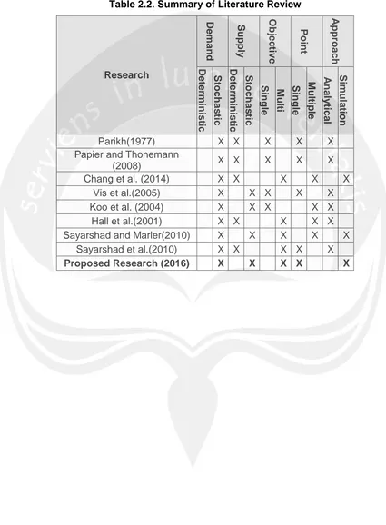
is not follows exponential distribution. The explanation of material inter-arrival time is explained in chapter 4. The summary of previous researches characteristic and research contribution can be seen in Table 2.2.
Table 2.2. Summary of Literature Review
Research D eman d S up ply O bjec tive P oint A pp roac h D eterm inis tic S toc ha sti c D eterm inis tic S toc ha sti c S ing le M ul ti S ing le M ul tip le A na lyti ca l S imul a tion
Parikh(1977) X X X X X Papier and Thonemann
(2008) X X X X X
Chang et al. (2014) X X X X X Vis et al.(2005) X X X X X Koo et al. (2004) X X X X X Hall et al.(2001) X X X X X Sayarshad and Marler(2010) X X X X X
Sayarshad et al.(2010) X X X X X