Agricultural and Forest Meteorology 114 (2003) 213–234
Spatial source-area analysis of three-dimensional moisture fields
from lidar, eddy covariance, and a footprint model
D.I. Cooper
a,∗, W.E. Eichinger
b, J. Archuleta
a, L. Hipps
c,
J. Kao
a, M.Y. Leclerc
d, C.M. Neale
c, J. Prueger
eaLos Alamos National Laboratory, Los Alamos, NM 87545, USA bUniversity of Iowa, Iowa City, Iowa, IA 52242, USA
cUtah State University, Logan, UT 84322, USA dUniversity of Georgia, Griffin, GA 30223, USA eNational Soil Tilth Laboratory, Ames, IA 50011, USA
Received 1 May 2001; received in revised form 23 August 2002; accepted 4 September 2002
Abstract
The Los Alamos National Laboratory scanning Raman lidar was used to measure the three-dimensional moisture field over a salt cedar canopy. A critical question concerning these measurements is; what are the spatial properties of the source region that contributes to the observed three-dimensional moisture field? Traditional methods used to address footprint properties rely on point sensor time-series data and the assumption of Taylor’s hypothesis to transform temporal data into the spatial domain. In this paper, the analysis of horizontal source-area size is addressed from direct lidar-based spatial analysis of the moisture field, eddy covariance co-spectra, and a dedicated footprint model. The results of these analysis techniques converged on the microscale average source region of between 25 and 75 m under ideal conditions. This work supports the concept that the scanning lidar can be used to map small scale boundary layer processes, including riparian zone moisture fields and fluxes. Published by Elsevier Science B.V.
Keywords:Spatial source-area analysis; Three-dimensional moisture; Latent energy flux
1. Introduction
The Los Alamos National laboratory (LANL) scanning Raman lidar has been used to measure mul-tidimensional water vapor fields for nearly a decade (Cooper et al., 1992). More recently, it has been used to estimate spatially resolved latent energy flux (LE) using a scalar gradient-based similarity ap-proach (Cooper et al., 2000; Eichinger et al., 2000). Three-dimensional fields of water vapor can be
trans-∗Corresponding author. Tel.:+1-505-665-6501;
fax:+1-505-667-7460.
E-mail address:[email protected] (D.I. Cooper).
lated into spatial estimates of surface fluxes if a known surface emitting region can be connected to the wa-ter vapor concentration at any particular height. This paper addresses the surface water vapor source-area sampling criteria and the extent of the flux footprint for application to remote sensing observations in the boundary layer. The sampling size depends on surface–atmosphere coupling and data acquisition properties, including the time required to scan over an area of interest. This study attempts to charac-terize lidar footprints and compare them with eddy covariance-derived co-spectra and a footprint model.
The “footprint issue” has been studied by inves-tigators for the past decade (Leclerc et al., 1997,
2003; Schuepp et al., 1990; Finn et al., 1996), and is a continuing topic of research. A number of dif-ferent approaches have been developed for both neutral and convective boundary layers using a: La-grangian model, large eddy simulation model, and analytical solutions to the advection–diffusion equa-tion (Leclerc et al., 1997). However, verification of the models with data has previously been limited to point sensors (Finn et al., 1996; Leclerc et al., 2003; Warland and Thurtell, 2000) or airborne line obser-vations (Ogunjemiyo et al., 1997). Since footprints and source-area concepts are inherently spatially de-pendent processes, multidimensional remotely sensed atmospheric data offer a unique opportunity to verify these models. Unlike other remote sensing systems, the scanning Raman lidar can spatially resolve atmo-spheric phenomena, especially within the boundary layer, and can thus be used to improve and perhaps verify boundary layer models (Kao et al., 2000). In turn, the footprint model results enhance the inter-pretation of lidar data and may help to improve lidar techniques in the field. The primary objective of this paper is to evaluate the optimum spatial sampling size for lidar derived variables such as latent energy flux.
In this paper, we first discuss the experimental site, the tower-based instruments used, and the scanning Raman lidar (Section 2). In next section (Section 3), we describe the Monin–Obukhov method for estimat-ing latent energy from lidar measured water vapor profiles and independent friction velocity measure-ments, as well as the dimensionless moisture flux,q∗.
Section 4describes three methods for estimating lidar average horizontal sampling size and point-source-area footprints by (A) combining lidar-eddy covari-ance, (B) footprint modeling analysis, (C) co-spectra of the vertical wind (w) and water vapor (q) time se-ries and (D) integral length scales. We finally discuss results and summarize inSection 5.
2. Site, instrument, and lidar overview
The study site was in the riparian corridor at the Bosque Del Apache Wildlife Refuge (hereafter called the Bosque) in the semi-arid south–central part of New Mexico, 25 km south of Soccoro, NM at ap-proximately 34◦N latitude, 107◦W longitude, at an
average elevation of 1376 m (Fig. 1). The Bosque is
adjacent to the Rio Grande river, which was flowing well during the experiment in mid-September 1998, due to the summer monsoon rains in late July. During the study period, the local climate was typically char-acterized by clear skies in the morning with stratocu-mulus clouds developing during the afternoon. Winds were generally mild at 2 m/s or less, northerly in the early morning, periodically the wind would reverse direction by mid-morning to become southerly. Wind directions subsequently oscillate between southeast and southwest throughout the day and through early evening transition hours. The vegetation at the Bosque consisted almost entirely of uniformly dense riparian
Tamarisk(salt cedar) 5 m tall with a height variation of±1 m. The Tamariskis a phreatophyte, thus water is not usually a limiting factor to evapotranspira-tion. The riparian corridor vegetation is adjacent to the western side of the river, covers a band between 500 and 700 m wide and extends north and south for several kilometers. During September the salt cedar canopy was closed with a green leaf area index of approximately two, as measured by a radiative LAI meter (Licor 2000).
Two 12 m tall micrometeorological towers were positioned between the western edge of the salt cedars and the Rio Grande, approximately 300 m from the river. The two towers were placed 685 m apart along the north–south direction. The following instruments were installed on the towers 2.7 m above the canopy: three-dimensional sonic anemometers (CSI Incorpo-rated CSAT-7),1 fine-wire thermocouples, Krypton
hygrometers (KH-20), temperature–humidity probes (Vaisala HMP100a), infrared thermometers (Everest), and net radiometers (REBS Q-7). Five soil heat flux plates (REBS) were buried 0.08 m below the soil sur-face and spatially distributed to represent the range of shade conditions below the canopy. Soil thermo-couples were located above the heat flux plates at
−0.02 and −0.06 m. The displacement heightd was estimated to be 0.6 the height of the vegetationh. Tur-bulent fluxes of sensible heat, latent heat, and momen-tum were computed using standard methods with a rotated re-sampled coordinate system from the above mentioned micrometeorological sensors using eddy covariance at 20 Hz (CSI Incorporated, 1998; Prueger
1Indication of manufacturer does not necessarily support an
D.I. Cooper et al. / Agricultural and Forest Meteorology 114 (2003) 213–234 215
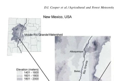
Fig. 1. Site map showing the location and elevation of the Bosque in relation to New Mexico and the study site in relation to the Bosque. The right panel is a false color image showing the salt cedar, cottonwoods, the drainage levee and the location of the micrometeorological towers and the lidar. The location of lidar scan azimuths forFig. 2A–Das well as the mean wind are shown as black lines on the IR image.
et al., 2000). In addition, an airborne visible/near IR imaging camera operated by the Utah State University collected images of the study site (Neal et al., 2000). A sand levee runs roughly north–south and the lidar, sodar, and profiling radar where located in the center of the levee (Fig. 1). The black strip shown west of the levee is the water in the drainage canal running par-allel to the Rio Grande. The open channel of the Rio Grande and the sand deposited on its banks are repre-sented by the high-reflectance patterns at the extreme east edge of the figure. The lidar was situated approx-imately at the midpoint between the two towers on the western edge of the salt cedar at the top of an adjacent levee. The levee was high enough that the lidar scan-ning mirror was approximately 3 m above the top of the canopy. An false-color image shows the relatively uniform, dense salt cedar canopy on the east and the
sparse cottonwoods on the west (Fig. 1). The lidar az-imuthal scan range covered 110◦from north to south,
and acquired data from the top of the canopy to 40 m into the atmospheric boundary layer (ABL). Several specific lidar scan azimuthal lines have been super-imposed on the false-color IR image shown inFig. 1
to illustrate the surface conditions for selected lidar observations. The LANL Raman lidar generates vol-ume images from multiple azimuth two-dimensional range-height-indicator scans of water vapor, hereafter called vertical scans. Details on the method and oper-ation of the scanning lidar are found inEichinger et al. (1999). We can operate the lidar to a radial range of about 600 m, a horizontal spatial resolution of 1.5 m, azimuthal scanning range up to 360◦, and a vertical
step resolution up to 0.05◦. Each vertical scan
increments from+35◦in azimuth to−145◦in azimuth
required about 15 min. The absolute accuracy of the li-dar was shown to be±0.34 g/kg at the 95% confidence level (Cooper et al., 1996; Eichinger et al., 1994).
3. Moisture fields and models for lidar
This section describes scalar observations over the Bosque and the present technique for flux esti-mation when locally available wind–field data are available. The Monin–Obukhov (M–O) length scale
L is a critical micrometeorological variable used to characterize local stability and estimate latent energy fluxes. The quantity L was derived for the Bosque site from wind–field measurements by a three-axis sonic anemometer eddy covariance sensor using the equation:
whereθvis the potential temperature,u∗is the friction
velocity,kis Von Karmen’s constant,g is the accel-eration due to gravity, and w′θ′
v is the sensible heat
flux. Monin–Obukhov similarity was used to estimate latent energy flux from the Bosque site by integrating wind–field and M–O data with lidar-derived water va-por profiles extracted from two-dimensional vertical scans (Eichinger et al., 2000).
3.1. Vertical scans and stability
Lidar vertical scans were typically between 500 and 600 m long and up to 40 m in height above the canopy top. The water vapor field over the Bosque was mea-sured by repeatedly scanning over the canopy directly
Table 1
Lidar scan acquisition and meteorological variables at 2.7 m above the canopy associated with selected figures Figure # DOY Time Az. (◦) θ
adjacent to the north tower and stepping in 5◦
az-imuthal increments from north to south, creating a well sampled three-dimensional water vapor field. Within any given 30 min period, between three and six ver-tical scans were recorded over the northern tower (at a 35◦ angle from the lidar) resulting in profiles that
were averaged in both space and time.
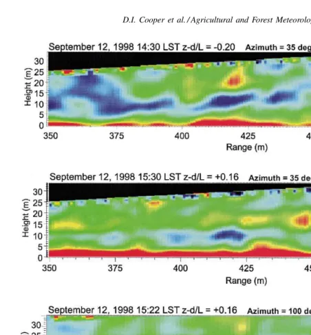
The vertical scans shown inFig. 2A and Billustrate the spatial structure of the ABL surface layer (lidar scan orientation relative to north and micrometeo-rological variables are listed in Table 1). Depending upon the prevailing stability conditions (as defined by
L), various structures are shown in the images: the
image generated from the vertical scan acquired dur-ing an unstable period shows the effects of convection and mixing, as the interaction of dry air from above and moist air from the surface produces intermittent microscale structures. In contrast, a vertical scan taken during a locally stable period shows a wetter region just above the canopy, as well as a region 10–15 m above the canopy surface that shows multiple moist microscale structures (red features) at about the same height (Fig. 2B). Earlier studies on forest–atmosphere interactions under convective conditions show multi-ple microscale structures at various heights (Cooper et al., 1994; Cooper et al., 2000). The 10 m tall structures between 10 and 15 m above the canopy in
D.I. Cooper et al. / Agricultural and Forest Meteorology 114 (2003) 213–234 217
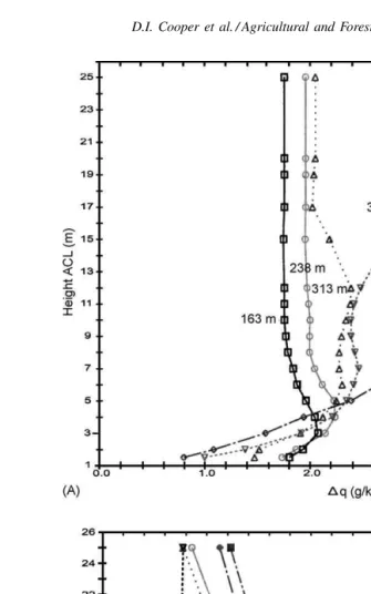
Each 500–600 m long range-height scan adja-cent to the north tower was sectioned into segments that can be defined as narrow as 5 m or as wide as 150 m in 1.5 m increments. The three-dimensional segments were then aggregated and plotted into two-dimensional profiles of water vapor versus height above the canopy. Depending on where the segment was extracted, the profiles extended up to 40 m above the canopy; the radial location along the scan deter-mines the total height due to the polar-coordinate (tri-angular shaped) range-height scanning pattern. These profiles were then corrected for terrain and canopy height using lidar-derived topographical information (Eichinger et al., 2000).
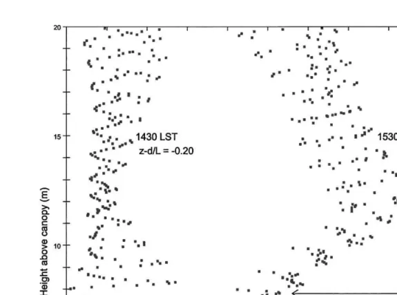
Vertical profiles of water vapor were extracted from two vertical scans shown in Fig. 2. These profiles were extracted from the region in the scans covering 350–375 m (±1.5 m of the north tower) the mix-ing ratio as a function of height is shown inFig. 3. The profile from the unstable period (z−d/L) = −0.20 shows a well-mixed lower surface layer with near-constant water vapor distribution above 5 m; be-low 5 m the distribution folbe-lows a curvilinear trend described by the classical Dyer–Hicks profiles for passive scalars (Monteith, 1973). Profiles displaying this shape are ideal for applying M–O similarity to estimate fluxes. In contrast, the profile extracted from the local stable period(z−d/L)= +0.16 is not only a wetter profile than the earlier example, but it also shows a moisture inversion between 7 and 13 m, indi-cated by the increase in moisture with height instead of the expected constant moisture profile. While the lower portion of the profiles (from 0 to 7 m) follows a curvilinear shape, the inversion above it sharply deviates from a log-normal water vapor distribution, limiting the application of M–O theory for these profiles to a few meters above the canopy (Fig. 3).
3.2. Lidar derived LE and q∗
The lidar elastic backscatter data are used to iden-tify both canopy geometry and topography since the backscatter from the canopy is several orders of mag-nitude larger than the Raman backscatter. The height of the canopy–surface water vapor observations were determined from the last high-value elastic-backscatter canopy-pixel from the lidar data. This height infor-mation is used to correct for topography and canopy
roughness variations (Eichinger et al., 2000). Water vapor versus height profiles are created from water vapor measurements that are taken over a range of a few centimeters above the canopy to tens of meters into the atmosphere (Cooper et al., 2000). The topo-graphically corrected water vapor profiles along with friction–velocity measurements are input into the clas-sical one-dimensional equation to estimate LE by the profile method (Brutsaert, 1982). The water vapor pro-file equation for latent energy is given by
LE=qz−q0(λku∗ρ)
where qz is the water vapor mixing ratio at some
height; q0 the surface water vapor mixing ratio; λ
the latent heat of vaporization; kthe Von Karman’s constant;u∗the friction velocity;ρ the air density; z
the measurement height; d the displacement height;
z0 the roughness length; ψsv(ζ)the stability
correc-tion and,w′q′ is the covariance of the vertical wind
with water vapor. In theory, the profile equation for LE flux should be equivalent to the eddy covariance derived flux, assuming that the source areas for the two techniques are similar (Wilson et al., 2001). A question outside the scope of this paper, but which will be addressed in the future is—in what region of space can au∗measurement observed at a point also be assumed to be valid for this technique? Recent re-search on the spatial variability of turbulent flux sug-gests that u∗ is less variable than LE (Katul et al., 1999).
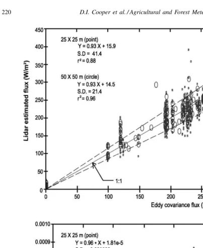
By utilizing lidar-measured high-resolution, spa-tially resolved profiles of mixing ratio and friction velocity measurements from a local three-dimensional sonic anemometer, spatially resolved fluxes were esti-mated with footprint diameters between 5 and 150 m centered over the north tower. A comparison of the eddy covariance fluxes versus lidar fluxes over several days is presented inFig. 4A. The plot shows that la-tent energy fluxes estimated by the two methods are in good agreement to within±15%, which is within the instrument uncertainty for eddy covariance-derived fluxes.
D.I.
Cooper
et
al.
/Agricultur
al
and
F
or
est
Meteor
olo
gy
114
(2003)
213–234
219
Fig. 4. Comparison of eddy covariance derived and lidar estimated LE (plot A) andq∗(plot B) for days of year 252, 254, and 255 with
D.I. Cooper et al. / Agricultural and Forest Meteorology 114 (2003) 213–234 221
the Monin–Obukhov derived fluxes (u∗). A more ro-bust analysis was used by partially eliminating u∗
from the estimate by calculating q∗ from Eq. (2)
as
It should be noted thatEq. (3)does not completely remove the effect of u∗ from the analysis since the stability correction employs the Monin–Obukhov length(L)and this requires a friction velocity
mea-surement. An eddy covariance-derivedq∗versus lidar
derivedq∗is shown inFig. 4B. Again, the plot shows
that lidar derived estimates forq∗ are within ±15%
of the point sensors. In addition, the analysis was performed for two footprint regions: 25 m×25 m and 50 m×50 m. Regression values suggest satisfactory slopes and small intercepts for both cases. Of interest is that the standard deviation of the regression and the coefficient of determination are better for the larger footprint, supporting the hypothesis that spatial sam-ple size plays an important role in the estimation of derived moisture quantities.
3.3. Advection, stability, and the effect of source area
Periodically in the mid-afternoon, the wind direc-tion would change from the north to the southwest. Westerly winds import dry warm air from the sparsely vegetated desert to the relatively moist, cool salt cedar canopy, creating locally stable atmospheres. Stability is determined here from eddy covariance measure-ments of L (Eq. (1)) where L is positive for stable
conditions and negative for unstable conditions. The effect of “hot to cold” advection on the stability of turbulent heat and moisture fluxes in semi-arid en-vironments is sometimes referred to as the “oasis effect.” The oasis effect is when hot dry air blows over a vegetated field in a desert, increasing transpira-tion and thus generating relatively cool moist air, such as at the Bosque. The dry air moving over the moist canopy increases the local vapor pressure deficit, in turn has a profound effect on the temperature gradi-ent and the sensible heat flux in that the direction of the gradient and thus the flux will change from
go-ing away from the surface to gogo-ing into the surface. The local advection equation relating the potential temperature gradient to the sensible heat flux is
u
A change in the direction of the flux was observed by the eddy covariance flux sensors over the salt cedar between 1430 and 1530 h on September 12,1998. In this 1-h period, the wind direction changed from northerly (parallel to the river) to southwesterly (from the desert into the Bosque) and, as expected when
L became positive, the sensible heat went into the
canopy, from+62 Wm−2at 1430 h to−22 Wm−2at
1530 h (seeTable 1).
The process of advection can account for some of the structures shown in Fig. 2B, as well as the afternoon stable conditions observed by the microm-eteorological instruments, and the moisture inversion shown in Fig. 3. Additional lidar and micrometeoro-logical data are used to support the hypothesis that the observed local stability is due to dry air transported over the Tamarisk canopy. For instance, in the lidar scan shown inFig. 2B, the high-moisture-containing structures (red features) located between 10 and 15 m above the canopy were observed during a locally sta-ble period (z−d/L >0). The false-color IR image of the site (Fig. 1) shows the location where scans 2B–D where taken as well as the direction of the mean wind during this period, and Table 1 lists the lidar scan orientations and associated micrometeorological vari-ables. These scans illustrate how the source of the rel-atively dry air that was advected over the canopy was ultimately the cause of the local stability and associ-ated moisture-containing structures found in the lidar data.
A lidar scan taken nearly perpendicular to the mean wind (Fig. 2C) shows the effect of dry air being ad-vected into the salt cedar, as the dynamic range of this data is approximately 50% higher than that shown in
This scan measured atmospheric moisture between 1 and 1.5 g/kg drier than those shown in Fig. 2B, re-flecting the relatively dry source area for this portion of the site.
From the footprint analysis that will be presented later in more detail (Section 4.2), for a stability of (z−d/L) = +0.16 the expected length of the source-area footprint will be about 450 m to achieve 90% of the cumulative water vapor flux. Using this footprint result, advected air from 193◦ moving
to-ward the region whereFig. 2Bwas acquired will be an admixture of high-moisture air from theTamariskand the dry air from the desert. This mixing is illustrated inFig. 2C which is intermediate between the “dry” scan of Fig. 2D and the “wet” scan ofFig. 2B. The moist structures occurring between 10 and 15 m high (Fig. 2B) have moisture concentrations up to 14 g/kg, while at similar heights in the dry scan (Fig. 2D), the structures have lower concentrations between 12 and 13 g/kg; the background moisture below these structures is drier still, with water concentrations be-tween 9.5 and 11 g/kg. Since the profiles extracted from Fig. 2B were only 25 m wide, and the cumu-lative flux at this width is about 45%, it is logical to assume that 55% of the air in these profiles are non-local.
The mixture of dry desert air 8 m above the
Tamarisk with the moist air rising from the canopy (Fig. 2C) has a moisture concentration between 10.5 and 11.5 g/kg; this relatively dry air was advected over the canopy creating the inversion conditions observed by the lidar-derived water vapor profiles (Fig. 3). From this analysis, we have shown that advection is one of the critical processes that is involved in the development of the local stable inversions observed in the data.
A theoretical structure for surface layer “hot to cold” advection was developed using potential temperature profiles as a function of distance between two sur-face roughness conditions, such as from bare soil to irrigated fields as outlined by Kaimal and Finnigan (1994). They predicted asDyer and Crawford (1965)
observed earlier, that an advective inversion develops above the canopy and the intensity of that inversion is a function of distance from the dry region into an irrigated field as measured with temperature profiles. The effect of stability and mass advection is also es-timated for water vapor where moisture variables are
substituted for thermal variables inEq. (4)as
¯
The development of advectively driven inversions under daytime convective conditions should be ob-servable in water vapor scalar profiles from lidar, from heat or moisture flux profiles, or from profiles ofq∗
usingEq. (5)(Kaimal and Finnigan, 1994).
Profiles of q∗ were created from the lidar and mi-crometeorological data collected within a selected 75 m wide section of the vertical scans shown inFig. 3
and coincident measuredu∗andLobservations from the north tower, using the similarity equation for non-dimensional moisture outlined in Eq. (2). Us-ing these derivedq∗ values, the right side ofEq. (5)
is solved directly as a function of height above the canopy. The first of these profiles was for a region that began near the inner edge of the riparian zone and progressed above theTamariskstand toward the eastern edge of the study site directly adjacent to the Rio Orande. Theq∗profiles inFig. 5Awere acquired
at 1430 h under convective conditions when L < 0. The unstable conditions are evident in the increasing values of q∗, as relatively small inversions are seen at 3–4 m above the canopy presumably where eddy mixing occurs between moist rising plumes and drier down-welling air. In contrast, when L > 0 (as in
Fig. 5B), dry air advection creates deep inversions 2–3 m above the canopy near the western edge of the
D.I. Cooper et al. / Agricultural and Forest Meteorology 114 (2003) 213–234 223
Fig. 5. Profiles ofq∗for day 256 during an unstable period at 14:30 LST (A), and for a stable period at 15:30 LST (B). Range values
4. Spatial analysis of sampling size
The standard sampling size for lidar derived LE flux estimates previously used an empirical 25 m×25 m region. However that sample size was found to under-estimate the flux; a 75 m×75 m footprint was found to produce better LE estimates (Cooper et al., 2000). To quantitatively determine the spatial extent of the average horizontal flux source area, four techniques were employed using lidar data, point-sensors derived time series data, and a model, (1) an analysis of lidar derived LE flux as a function of source-area size; (2) an analysis ofwandqspectra from local eddy co-variance measurements; (3) analysis from a footprint model; and (4) integral length scales.
4.1. Normalized flux and horizontal average length
To evaluate the individual weighted contributions from sources at different positions throughout the lidar field-of-view and to infer the total spatial flux of that region, we truncated the range-height scans for differ-ent lengths and examined the fractional contribution to the flux as a function of the horizontal sampling length.
The gradient-based M–O latent energy estimation method for lidar requires input ofu∗,L, air density,
and a segment of lidar data extracted from a series of vertical scans averaged and interpolated over space and time (seeSection 3.1). From these data, a profile of water vapor is generated and fitted with a M–O-derived water vapor distribution estimate, allowing latent en-ergy and q∗ to be calculated, as well as a coeffi-cient of determination (r2) for the best-fit between the lidar-derived moisture profile and the M–O-predicted profile.
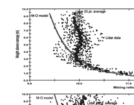
Examples of vertical profiles fitted with an M–O water vapor distribution are shown in Fig. 6. These plots show the lidar data as points, a 20-point smoothed profile as large filled circles, and the model as a thick line. It appears from the two examples that the M–O-derived profiles are somewhat drier above 4 m than the lidar derived moisture distributions. This dry bias is clear in a comparison of the 20-point smoothed profile and the M–O-derived distribution, as they significantly diverge (differences≥0.25 g/kg) above 5 m. The for the best-fit for the two examples is shown in the upper right-hand corner of each plot.
The upper panel has anr2of 0.93 for a 50 m diameter footprint; in contrast, ther2for a 90 m diameter foot-print is considerably lower at 0.77. These statistics are almost counter-intuitive, as the expected result would be that the larger the number of data points averaged together, the better the fit. The effect of spatial sample size can also be seen in the smoothed profile, as the large horizontal sample length pro-file shows considerable variability when compared with the 50 m diameter sampling length profile. The degraded fit for the larger footprint indicates that over-sampling (1) is reflected in the spatial variability of the vertical profile moisture by 50% larger dy-namic range of mixing ratio; (2) does not alleviate the dry bias of M–O derived profiles when compared with lidar-derived profiles and (3) does not appear to improve flux estimates relative to those made from tower-based measurements. Following McNaughton and Laubach (2000), the dry bias in the M–O-derived profile appears to result from moist microscale con-vective eddies rising from the surface and mixing with advected dry air that is representative of the arid regions surrounding the Bosque (see Section 3.2). To evaluate optimal horizontal source-area averages for lidar-based latent energy estimates, we performed spatial analyses using a ratio of lidar derived fluxes to tower-based flues (normalized flux).
A normalized LE flux (LEN) was calculated as
LEN(LHL)=
LEL LET
r2 (6)
where LEL is the M–O-derived LE flux for a given
horizontal lidar flux sampling length (LHL),LETis the
tower-based eddy covariance-derived flux, and r2 is the coefficient of determination derived from the M–O best-fit to the lidar-derived moisture profile. We note that different LHL’s can in some cases produce the
same lidar derived flux estimate. However, because the quality of the fit between the theoretical M–O profile and the actual data varies substantially (SeeFig. 4),r2
can be used as a weighting factor to separate similar flux values with differing fits. The set of LHL’s used
in this study was from 5 to 105 m in 10 m increments or lags.
D.I.
Cooper
et
al.
/Agricultur
al
and
F
or
est
Meteor
olo
gy
114
(2003)
213–234
225
D.I.
Cooper
et
al.
/Agricultur
al
and
F
or
est
Meteor
olo
gy
114
(2003)
213–234
D.I. Cooper et al. / Agricultural and Forest Meteorology 114 (2003) 213–234 227
diverging values from the tower-based eddy covari-ance ‘truth-set’.
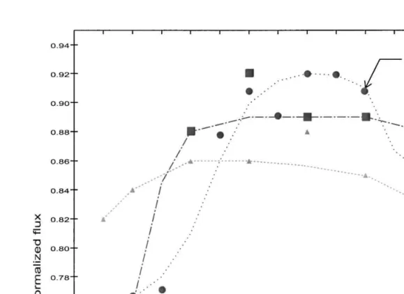
Using the normalized flux, we evaluated the hori-zontal average sample length of LE over two orders of magnitude, from between 5 and 100 m, and over various stability conditions (Fig. 7). We found that for relatively unstable (z−d/L) values (−0.48), the LE source area appears to be relatively broad. In contrast, small (z−d/L) values (−0.13) influence the horizontal averaging length, exhibiting a more pronounced and narrow normalized-flux region. Further, under stable conditions, when (z−d/L= +0.16), the horizontal averaging length appears, to be both broader and flat-ter then the curves derived under unstable conditions. From this analysis, we conclude that as the convective activity decreases, surface–atmosphere coupling de-creases, leading to lower normalized fluxes at larger horizontal average lengths (>80 m). Furthermore, as convection decreases, it appears that the source region increases in size. At more modest lengths, 30–60 m, the source area was better matched to the rough-ness elements and wind speed thus optimizing the surface–atmosphere coupling, which in turn leads to high-normalized flux values. If the lags are too small, there will not be enough data to generate a statistically reliable flux value. These analyses suggest that 40 m×
40 m (1600 m2) to 60 m×60 m (3600 m2) sample size at 30 min averaging periods is reasonable for flux map-ping in uniform terrain conditions. These empirical, lidar-data-based results are comparable to those from footprint models, as described in the next section.
4.2. Theoretical footprint analysis
We used a Lagrangian model described extensively in the literature to predict the water vapor mixing ratio profile, latent energy flux, and footprints for a crosswind line source within the surface layer of the ABL (Leclerc et al., 1997). These flux footprints were estimated from the upwind sources of moisture that would be measured at a point in space with the cross-wind integrated probability density function of mois-ture transported from the surface (Baldocchi, 1997; Leclerc et al., 1997). The vertical eddy flux density,F
is defined as
F (x, z)= x
0
Q(x′)f (x′, z)dx′ (7)
where x is the stream-wise distance, z the observa-tion or measurement height, x′ the upwind distance,
Q(x′) the upwind surface source density, and f(x′,
z) is the crosswind-integrated footprint probability density function. We note that the general footprint calculation used here Eq. (7) also includes specific corrections for atmospheric stability. Specific numer-ical solutions to f(x′, z) are found in Leclerc et al.
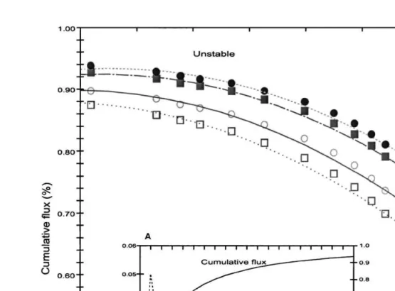
(1997); Leclerc and Thurtell (1990) and Schuepp et al. (1990)describing the original work on the sub-ject. A plot of the relationship between (z−d/L) and the cumulative flux is shown in Fig. 8, where each symbol represents a selected downwind distance or lag as a function of (z −d/L) and cumulative flux, and the lines connecting the points are sec-ond order polynomial best-fits. As the atmosphere becomes more convectively active, the footprints be-come smaller; at (z −d/L) = −0.6, 90% of the cumulative LE flux is within a 60 m diameter source region. Conversely, at(z−d/L)= −0.1, 81% of the cumulative LE flux is accounted for within a 90 m diameter footprint. Further, under stable conditions the footprints become considerably larger and the cu-mulative flux for a given footprint becomes relatively small when compared with unstable conditions in the surface layer. By extrapolating the family of curves shown in Fig. 8 to increasingly unstable conditions, the cumulative flux reaches an asymptote at 93% when (z−d/L) = −1.1 suggesting that there is a limit to the effect of vertical coupling on footprint size.
Flux footprints were calculated for a series of L,
u∗ and wind–field values measured at the Bosque. In modestly convective conditions, such as when
L = −10 and (z−d/L) = −0.48, the footprint lag length (analogous to the LHD) was between 40
D.I.
Cooper
et
al.
/Agricultur
al
and
F
or
est
Meteor
olo
gy
114
(2003)
213–234
D.I. Cooper et al. / Agricultural and Forest Meteorology 114 (2003) 213–234 229
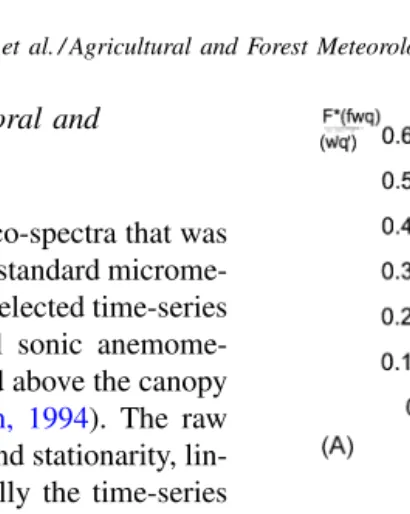
4.3. Co-spectra analysis for temporal and spatial scales
For the construction of relevant co-spectra that was coincident with lidar data, we used standard microme-teorological techniques to process selected time-series values from the three-dimensional sonic anemome-ter and Krypton hygromeanemome-ter located above the canopy (Stull, 1988; Kaimal and Finnigan, 1994). The raw data were screened for continuity and stationarity, lin-ear trends were removed, and finally the time-series data were multiplied by a tapered window to create a conditioned time series data set. The conditioned data set consisted of 20 Hz sampled values ofu,v,w, and
q. The data were transformed from time-domain to frequency-domain by discrete Fourier analysis. Spec-tral density distributions for water vapor and verti-cal wind were computed, and periods of interest were further processed into the co-spectra. The co-spectra were normalized by the covariance of w and q for the comparison of frequency between various times (Prueger et al., 2000). Frequency information from the co-spectra were transformed into the spatial domain by invoking Taylor’s hypothesis by assuming that the temporal turbulence statistics are equivalent in space as:
1
fu¯2π (8)
wherefis the co-spectra frequency, u¯ is mean wind, and 2π is used to convert from angular to linear di-mensions.
The co-spectra results were used to evaluate the temporal and spatial length scales associated with the fractional contribution to latent energy flux. We assumed that spatial and temporal length scales as-sociated with co-spectra are directly related to the source-area contribution to the flux integrated in time over 30 min.
Two sample co-spectra with (z−d/L) of −0.20 (Fig. 8A) and +0.16 (Fig. 8B) illustrate some of the surface–atmosphere processes occurring at the Bosque. The results shown inFig. 9A are typical of the unstable conditions reflected by the co-spectra pro-cessed from the Bosque data set. The peak frequency is approximately 0.04 s−1; when translated into
tem-poral and spatial scales, the peak represents 25 s and 191 m, respectively. The bulk of the energy-containing
Fig. 9. Co-spectra ofwandqacquired from the north tower eddy covariance-time series during selected unstable (A) and stable (B) periods.
length scales were between 50 and 200 m, with little contribution above 225 m. Spectra from locally stable periods shown in Fig. 9B were somewhat different from the unstable periods. The frequency for peak power density was lower at 0.0263 s−1 or 38 s and
et al. (2000) found that the lidar can be used to re-solve plumes and eddies with reasonable statistical and physical accuracy even though the scan rate is rel-atively slow. From the co-spectra shown in Fig. 8A and B, it appears that eddy lengths between 190 and 274 m were responsible for peak fractional fluxes. The dominant eddies contributing to the flux were on the order of 10–200 m in diameter, while eddies range from 500 to 1000 m in diameter made minor contribu-tions to the total flux. The time-series analysis ofwq
co-spectra suggests that the source areas for LE are microscale, supporting the results of the footprint and lidar-based analyses of sample size region.
4.4. Integral length scales
Integral time and spatial scales were estimated from moisture observations with both tower-based time series and lidar-based spatial series to determine the length and time of eddy and plume coherency. The Eulerian integral length scale Λ is traditionally derived from the Lagrangian integral time scale τ
and multiplied by the mean wind to estimate a spatial scale (Hanna, 1981). Because lidar data are acquired by a spatially fixed instrument that are range-resolved, the mean wind is not required, allowing the spatial scale to be computed directly. The τ can be esti-mated from the autocorrelation function of a variable when the lag is equal to l/e, if the time-series PDF is near-Gaussian and the autocorrelation function can be integrated to infinity (Kaimal and Finnigan, 1994; Pope, 2000). Thus, the Eulerian integral length scale for water vapor is
Λq= ¯uτq= ¯u ∞
0
ρq(ξ ) (9)
where the autocorrelation function for water vapor is
ρq(ξ )= qi′qi′+ξ
σq2 (10)
and the conditional water vapor estimates are
qi′=qi− ¯qi qi′+ξ =qi+ξ− ¯qi+ξ (11)
whereiin this case is an individual water vapor value
q, at some range (for lidar data) or time (for Krypton hygrometer data) and ξ is the lag in range or time. The integration of autocorrelation functions for water
vapor over infinite spatial or temporal lags is not pos-sible, and for convenience we assumed that the finite sampled population is adequate. Furthermore, the l/e integrating limit does not work for high-frequency variables such as 20 Hz measuredqvalues, since the autocorrelation curves tend to have complex shapes, instead the first zero crossing of the autocorrelation function was chosen as the integrating limit (Kaimal and Finnigan, 1994).
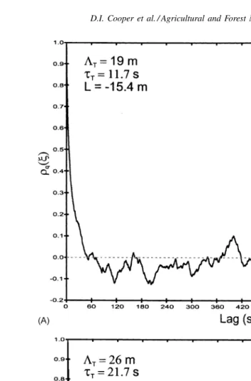
We calculated autocorrelation functions from wa-ter vapor measurements from the lidar and Krypton hygrometer for both unstable and stable conditions. Lidar range-resolvedqtransects 500 m long were ex-tracted from horizontal lines-of-sight 2.7 m above the canopy where the tower-based sensors were located. Further, 10-min-long time-series ofqvalues were ex-tracted from the Krypton hygrometer data taken at the same time as the lidar data so we could also estimate the integrated length scale. The spatial and temporal series were normalized by first detrending the data using a least-squares linear fit and then smoothed using a Savitzky–Golay filter (Press et al., 1989); the normalized data were then input intoEq. (9).
The results of the autocorrelation processing are shown in Fig. 10, where panels A and C are from the unstable case from the Krypton hygrometer and the lidar, respectively, while panels B and D are for the stable case. The unstable cases (panels A and C) show that the integral length scales are under 20 m. In contrast, the stable cases (panel B and D) show that the length scales are larger, somewhat over 25 m. The integral time scales show that the time scale for unstable periods (11.7 s) is substantially shorter than for stable cases (21.7 s), since the unstable regime is better mixed, reducing the lifetime of the eddies.
The integral temporal and length scales are a char-acteristic property of the water vapor eddy structure and should be related to source properties such as roughness, stability, and spatial extent. The footprint analyses described in Section 4.2 indicate that peak fractional fluxes occur under 10 m regardless of sta-bility (Fig. 8), while the cumulative flux analyses show that stable footprints are considerably larger than unstable cases, which is also supported by theΛ
D.I. Cooper et al. / Agricultural and Forest Meteorology 114 (2003) 213–234 231
D.I. Cooper et al. / Agricultural and Forest Meteorology 114 (2003) 213–234 233 5. Conclusions
The lidar-based estimates of water vapor flux were in good agreement with tower-based eddy covariance measurements, indicating that the technique works well under the conditions prevalent at the Bosque. The footprint analyses suggest that the spatial varia-tions observed in the fluxes appear reasonable but are specific to the height-roughness elements and stability regimes evaluated in this study.
The results of the analyses presented in this pa-per indicate that the spatial sampling size used for lidar-derived fluxes should be between 25 and 75 m in diameter. Comparisons of lidar-derived LE estimates and tower-based eddy covariance measurements sug-gest that the optimum spatial footprint is between 40 and 60 m under low windspeed conditions and a close canopy. Footprint estimation by Lagrangian dispersion modeling techniques also suggests that 40–60 m is a reasonable spatial sampling size. Lidar spatial sample size is partially dependent on local stability conditions as defined by (z−d/L), however other factors such as roughness elements and surface homogeneity also play an important role in sampling strategy.
This work is an initial step in improving our under-standing of the spatial sampling requirements as the analyses was performed on data acquired under ideal conditions of large, homogeneous closed canopy, uni-form height and roughness on nearly level terrain. Re-search on less-optimal environments and conditions will be performed in the future to determine if these techniques can be extended to more complex terrain and heterogeneous vegetation. However, the analyses presented in this study points to spatial scales for hydrological and boundary layer interactions that are occurring at micrometeorological scales.
The data from the Bosque experiment suggest that relatively small mapping units (i.e. the source region), under 100 m, appear to be sufficient when surface roughness is uniform indicating that modest fields can be spatially resolved if other factors such asu∗
variability are small. It also appears that optimal lidar spatial sample sizes and the footprint analysis are in good agreement with one another. The footprint anal-ysis suggests that increasing sample size improves flux estimates, in contrast spatial variability analysis suggests that sample size limits are necessary. To-gether, these findings suggest that there is an optimum
sampling size. In future field programs, the analysis of lidar mapping unit size should be determined by using some form of footprint analysis. In addition, the idea that trading space for time appears to be a reasonable assumption in these kinds of environments, further supporting the use of remote sensing as a quantitative tool in surface–atmosphere studies. The reasonable flux estimates resulted from profiles that were only short time averages, perhaps these good results are related to the fact that they are also averages in space. It is possible that the combination of space and time information is sufficient to provide a surrogate for the formally required ensemble average.
Acknowledgements
We would like to thank A. Fernandez, K. Vigil, and A. Reeves of LANL, Steve Hansen of the Bureau of Reclamation and his staff. Further, we would like to acknowledge the time and effort of the staff of the Bosque Del Apache Wildlife Refuge for making the site available. This work was performed and funded in part under DOE grant W7405-ENG-36.
References
Baldocchi, D., 1997. Flux footprints within and over forest canopies. Bound. Layer Meteorol. 85, 273–292.
Brutsaert, W., 1982. Evaporation into the Atmosphere. Theory, History, and Applications. Reidel, p. 299.
CSI Incorporated, 1998. CSAT3 Three-Dimensional Sonic Anemometer Instruction Manual. Campbell Scientific Inc., Logan, UT, USA, p. 26.
Charnay, G., Schon, J.P., Alcaraz, E., Mathieu, J., 1979. Thermal characteristics of an internal boundary layer with an inversion of wall heat flux. In: Durst, F., Launder, B.E., Schmidt, R.W., Whitelaw, J.H. (Eds.), Turbulent Shear Flows I. Spinger-Verlag, New York, pp. 104–118.
Cooper, D.I., Eichinger, W.E., Hipps, L., Kao, J., Reisner, J., Smith, S., Schaeffer, S.M., Williams, D.G., 2000. Spatial and temporal properties of water vapor and flux over a riparian canopy. Agric For. Meteorol. 105, 263–285.
Cooper, D.I., Eichinger, W.E., Barr, S., Cottingame, W., Hynes, M.V., Keller, C.F., Lebeda, C.F., Poling, D.A., 1996. High resolution properties of the equatorial pacific marine atmospheric boundary layer from lidar and radiosonde observations. J. Atmos. Sci. 53, 2054–2075.
Cooper, D.I., Eichinger, W.E., Holtkamp, D., Karl, R., Quick, R., Dugas, W., Hipps, L., 1992. Spatial variability of water vapor turbulent transfer within the boundary layer. Bound. Layer Meteorol. 61, 389–405.
Dyer, A.J., Crawford, T.V., 1965. Observations of climate at a leading edge. Quart. J. Roy. Meteor. Soc. 91, 345–348. Eichinger, W.E., Cooper, D.I., Chen, L.C., Hipps, L., Kao, C.-Y.J.,
2000. Estimation of spatially distributed latent heat flux over complex terrain from a Raman lidar. Agric For. Meteorol. 105, 238–261.
Eichinger, W.E., Cooper, D.I., Forman, P.R., Griegos, J., Osborn, M.A., Richter, D., Tellier, L.L., Thornton, R., 1999. The development of Raman water-vapor and elastic aerosol lidars for the central equatorial pacific experiment. J. Oceanic Atmos. Tech. 16, 1753–1766.
Eichinger, W.E., Cooper, D.I., Archuletta, F., Hof, D., Holtkamp, D., Karl, R., Quick, C., Tiee, J., 1994. Development and Application of a Scanning, Solar-Blind Water Raman-Lidar. Appl. Opt. 33, 3923–3932.
Finn, D., Lamb, B., Leclerc, M.Y., Horst, T.W., 1996. Experimental evaluation of analytical and Lagrangian surface-layer flux footprint models. Bound. Layer Meteorol. 80, 283–308. Hanna, S.R., 1981. Lagrangian and Eularian time-scale relations
in the daytime boundary layer. J. Appl. Meteorol. 20, 242–249. Kaimal, J.C., Finnigan, J.J., 1994. Atmospheric Boundary Layer
Flows. Oxford Press, New York, p. 289.
Kao, C.-Y.J., Hang, Y.-H., Cooper, D.I., Smith, W.S., Reisner, J.M., 2000. High resolution modeling of lidar data: mechanisms governing surface water vapor during SALSA. Agric. For. Meteorol. 105, 185–194.
Katul, G., Hsieh, C.I., Bowling, D., et al., 1999. Spatial variability of turbulent fluxes in the roughness sublayer of an even-aged pine forest. Bound. Layer Meteorol. 93, 1–28.
Leclerc, M.Y., Thurtell, G.W., 1990. Footprint predictions of scalar fluxes using Markovian analysis. Bound. Layer Meteorol. 53, 247–258.
Leclerc, M.Y., Shen, S., Lamb, B., 1997. Observations and large eddy simulation modeling of footprints in the lower convective boundary layer. J. Geophys. Res. 102, 9323–9334.
Leclerc, M.Y., Karipot, A., Prabha, T., Aliwine, G., Lamb, B., Gholz, 2003. Experimental evaluation of flux footprint
models over a forest canopy and effects of larger-scale advection on tracer fluxes. Agric. Forest Meteorol. (submitted for publication).
McNaughton, K.G., Laubach, J., 2000. Power spectra and co-spectra for wind and scalars in a disturbed surface layer at the base of an advective inversion. Bound. Layer Meteorol. 96, 143–185.
Monteith, J.L., 1973. Principles of Environmental Physics. Arnold, p. 241.
Neal, C.M., Hipps, L., Prueger, J.H., Kustas, W.P., Cooper, D.I., Eichinger, W.E., 2000. Spatial mapping of evapotranspiration and energy balance components over riparian vegetation using airborne remote sensing. In: Owe, M., Brubaker, K., Ritchie, J., Rango, A. (Eds.), Remote Sensing and Hydrology, Pub. No. 267, IAHS, pp. 233–238.
Ogunjemiyo, S., Schuepp, P.H., MacPherson, J.I., Desjardins, R.L., 1997. Analysis of flux maps versus surface characteristics from Twin Otter grid flights in BOREAS 1994. J. Geophys. Res. 102, 29135–29145.
Pope, S.B., 2000. Turbulent Flows. Cambridge University Press, Cambridge, p. 771.
Press, W.H., Flannery, B.P., Teukoisky, S.A., Vetterling, W.T., 1989. Numerical Recipes, 2nd ed. Cambridge University Press, Cambridge, p. 973.
Prueger, J.H., Hipps, L.E., Hatfield, J.L., Kustas, W.P., 2000. Turbulence characteristics in a dense riparianTamariskcanopy. In: Proceedings of the 24th Conference on Agricultural and Forest Meteorology, AMS, Boston MA, pp. 204–205. Schuepp, P.H., Leclerc, M.Y., Macpherson, J.J., Desjardins, R.L.,
1990. Footprint prediction of scalar fluxes from analytical solutions of the diffusion equation. Bound. Layer Meteorol. 50, 355–373.
Stull, R., 1988, An Introduction to Boundary Layer Meteorology, Kluwer Academic Publishers, Boston, MA, p. 666.
Warland, J.S., Thurtell, G.W., 2000. A Lagrangian solution to the relationship between a distributed source and concentration profile. Bound. Layer Meteorol. 96, 453–471.