Haze Modelling and Simulation in Remote Sensing Satellite Data.

http://dx.doi.org/10.12988/ams.2014.49761

Haze Modelling and Simulation in Remote

Sensing Satellite Data

Asmala Ahmad

Department of Industrial Computing

Faculty of Information and Communication Technology Universiti Teknikal Malaysia Melaka

Hang Tuah Jaya, 76100 Durian Tunggal, Melaka, Malaysia Shaun Quegan

Department of Applied Mathematics School of Mathematics and Statistics

University of Sheffield Sheffield, United Kingdom

Copyright © 2014 Asmala Ahmad and Shaun Quegan. This is an open access article distributed under the Creative Commons Attribution License, which permits unrestricted use, distribution, and reproduction in any medium, provided the original work is properly cited.

Abstract

In atmospheric haze studies, it is almost impossible to obtain remote sensing data which have the required haze concentration levels. This problem can be overcome if we can generate haze layer based on the properties of real haze to be integrated with remote sensing data. This work aims to generate remote sensing datasets that have been degraded with haze by taking into account the spectral and spatial properties of real haze. Initially, we modelled solar radiances observed from satellite by taking into consideration direct and indirect radiances reflected from the Earth surface during hazy condition. These radiances are then simulated using the 6SV1 radiative transfer model so that the radiances due to haze, or the so

Keywords: Haze, Modelling, Simulation, Landsat, Radiance

1 Introduction

Atmospheric aerosols and molecules scatter and absorb solar radiation, thus affecting the downward and upward radiance. Atmospheric scattering and absorption depend substantially on the wavelength of the radiation [16]. Scattering is usually much stronger for short wavelengths than for long wavelengths and significantly affects the classification of surface features [3], [17]. Studies related to haze effects on remote sensing measurements commonly use real hazy datasets [6], [10], [14]. However, acquiring real hazy datasets with a desired range of haze concentrations over an area is almost impossible [1]. A more practical way is to model the haze and simulate its effects on satellite dataset. To do so, we need to know the effects that haze concentrations have on scene visibility and to translate it onto real remote sensing data. An important issue in realising this is to model hazy dataset [16]; in section 2, a model for integrating haze with a clear atmosphere dataset is described. Next, we need to translate the model to practical processes [15]; section 3 discusses radiance calculation using the 6SV1 model. Haze spatial distribution is another key issue in generating real haze [17]; section 4 discusses representation of haze spatial properties using multivariate Gaussian distribution. Finally, the most critical task is to integrate haze layer with a real dataset in order to produce a hazy dataset [12]; section 5 discusses simulation of hazy datasets by incorporating simulated haze path radiance, the effects of signal attenuation and haze spatial distribution onto a clear dataset.

2 Model for Determining Satellite Observed Radiance under Hazy

Conditions

The observed radiance,L_{, that reaches the sensor for a cloudless and haze-free}

atmosphere can be expressed as [16]:

S D O

L L L L ... (1)

where L is the radiance reflected by the target and directly transmitted through _S the atmosphere towards the satellite (this gives most information about the target

on the Earth’s surface), L is the radiance reflected from the surface and then D scattered by the atmosphere to the sensor (this diffuses radiation between different pixels and thus reduces the spatial variation of the upward radiance), and L is _O

the radiance scattered into the sensor’s field of view by the atmosphere itself (caused by the atmospheric constituents that exist during clear sky conditions)

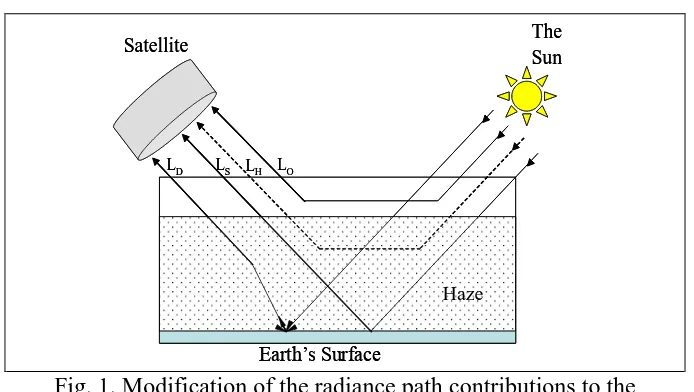
the image brightness. To account for haze, Equation (1) is modified as follows (Figure 1):

S D O H

L L L L L ... (2)

where L is the radiance caused by the haze layer. It is independent of the surface _H reflectance and increases image brightness for dark targets, but decreases it for bright targets. Similarly, Equation (2) can also be expressed as:





S D O H S D P

L L L  L L  L L L ... (3)

where L_P L_OL_H is known as path radiance.

Satellite The

Sun

LO

LS

LD LH

Earth’s Surface

Satellite The

Sun

LO

LS

LD LH

[image:3.595.125.472.332.528.2]

Earth’s Surface

Fig. 1. Modification of the radiance path contributions to the satellite sensor in hazy conditions.

The contribution of LD is insignificant since it is much weaker than the other

components [17] and therefore can be neglected, hence:





S O H S P

L L L L  L L ... (4)

We introduce a model for simulation of hazy data in which Equation (4) is written as:

 



 1

 



 

 2

   

S O H

L V  1 β V L  _L β V L 0 _ ... (5)

where L_S

 

V  



1 β V L 1

 



_S

 

 and L (V)_P L_Oβ 2

   

V L 0_H . V is the visibility, L V is the target radiance at visibility V km, so

 

L_S

 

 is the radiance

of pure target (i.e. the atmospheric components are assumed insignificant),

 

H

L 0 is for pure haze and the weightings β V 1

 

and β 2

 

V are given by:

 

 

 

 

1 S

S

L V

β V 1

L

 

 ... (6)

 

 

 

 

2 P O

H

L V L

β V

L 0



 ... (7)

In Equation 5, during a clear day,V ,β 1

 

 β 2

 

 0, therefore

 

S

 

O

L  L  L . For very thick haze,V0_,β 0 1

 

β 2

 

0 1 , so

 

O H

 

L 0 L L 0 . In other words, during clear and very hazy conditions, the radiance observed by the satellite sensor is actually the radiance of true signal and pure haze respectively added with L . Between the two extremes, _O L_S

 

V is influenced by



1β V 1

 



due to atmospheric absorption, while L_P

 

V is influenced by β 2

 

V due to atmospheric scattering. We can estimate L_S

 



from a clear Landsat satellite dataset, while determination of L_H

 

_{0 ,} β V 1

 

and

 2

 

β V are discussed in the following section.

3 Radiance Calculation Using the 6SV1

6SV1 is the vector version of the 6S (Second Simulation of the Satellite Signal in the Solar Spectrum) [15], [12], though it also works in scalar mode. The vector version is introduced to account for radiation polarisation, due to Rayleigh scattering in a mixed molecular-aerosol atmosphere, which is to be used when performing atmospheric correction [15]. In our study, the 6SV1 is used in simulating haze effects, therefore the radiation polarisation effect is assumed negligible. Hence, our interest is in the scalar mode of 6SV1, which is similar to 6S. 6S makes use of the Successive Order of Scattering (SOS) algorithm to calculate Rayleigh scattering, aerosol scattering and coupling of scattering-absorption. In the SOS, the atmosphere is divided into a number of layers, and the radiative transfer equation is solved for each layer with an iterative approach [12], [15]. In terms of the aerosol model, a refined computation of the radiative properties of basic components (e.g. soot, oceanic, dust-like and water soluble) and additional aerosol components (e.g. stratospheric, desertic and biomass burning) is included. It also has a spectroscopic database for important gases in

Lambertian and non-Lambertian targets. For a Lambertian uniform target, the apparent radiance ρ* is calculated using [12]:









   

* t

s v s v a r s v s v s v

t

, , , , T T

1 S

 

 

             

 ... (8)

where _{a r}



   _s, _v, _{s v}



is the intrinsic atmospheric reflectance associated with aerosol (a) and Rayleigh scattering (r), t is the surface reflectance, S is the atmospheric spherical albedo, T

 

s

 _{ is the total downward transmission and}

 

v

T  is the total upward transmission. _s and _v are the solar and satellite zenith angle respectively and s and v are solar and satellite azimuth angle respectively.

 

s

 

s d s

T  e  t ... (9)

 

v

 

v d v

T  e  t ... (10)

where     a r is the atmospheric optical thickness associated with aerosol (a) and Rayleigh scattering (_r), μ_s and μ_v are cos

 

θ_s and cos

 

θ_v respectively and t is the diffuse transmittance due to molecules and aerosols. Substituting _d (10) into (8), we have:









 

s v

 

*

s v s v a r s v s v t t d v

t T

, , , , e t

1 S

 _



   

            _   _

   ... (11)

For a non-uniform surface:









 

s v

 

*

s v s v a r s v s v t e d v

e T

, , , , e t

1 S

 _



   

            _   _

   ... (12)

where e is the environmental reflectance and can be expressed as:

   

2

e _{0 0}

dF r 1

r, dr d

2 dr

 

    

The intrinsic atmospheric reflectance,_{a r}



   _s, _v, _{s v}



, is computed using:





'





s v

 

a r s, v, s v a r s, v, s v 1 e 1 e

 

 _  _

    

            _{ }  _ 

   ... (14)

where 'a r



   s, v, s v



is the single-scattering contribution associated with aerosol and molecule scattering and _{1 e} s _{1 e} v

 

 

 _  _

 _  _ _{ }

  

   accounts for

higher orders of scattering. The atmospheric spherical albedo S is calculated using:

 

 

3 4

1

S 3 4E 6E

4 3  

 _     _

  ... (15)

where E₃

 

 and E₄

 

 are exponential integrals depending on . To exploit Equation (5), we need to determineL_H

 

0 , β V 1

 

andβ 2

 

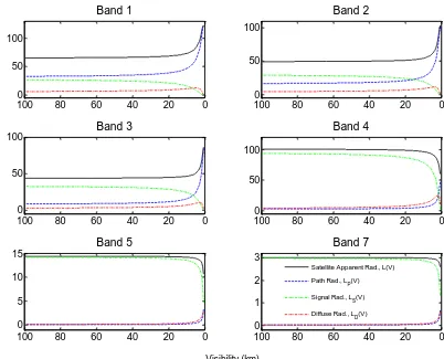
V . To do so, we use the 6SV1 code to calculate satellite apparent radiance, path radiance, signal radiance and diffuse radiance, for bands 1, 2, 3, 4, 5, and 7 of the Landsat satellite. The atmospheric and aerosol model used were Tropical Model and Biomass Burning respectively. The latter accounts for haze that originates from forest fires. Initially, visibility was varied from 0.5 to 100 km, but later only visibilities from 0.5 to 20 km were taken into account. The following section further explains this issue. Figure 2 shows satellite apparent radiance, path radiance, signal radiance and diffuse radiance as a function of visibility. It is obvious that for bands 1, 2 and 3, the path radiance is higher than the diffuse radiance at all visibilities. For bands 4, 5 and 7, the path and diffuse radiance are about the same but the signal radiance is comparatively much higher. This shows that at shorter wavelengths the haze effects are significant and dominated by the path radiance; while at longer wavelengths, the haze effects are almost negligible due to the much higher signal radiance. It is also observed that the major impact on the radiances occurs for visibilities less than 20 km. Hence, we make the approximations L_S

 

 L_S

 

20 andL_P

 

 L_OL_P

 

20 . Also, in 6SV1, calculations cannot be made for visibilities less than 0.5 km, so we assume L 0_S

 

L 0.5_S

 

and

 

 

 

P P O H

L 0 L 0.5 L L 0.5 . Thus, Equation 5 can be written as:

 



 1

 



 

 2

   

S O H

0 20 40 60 80 100 0 50 100 Band 1 0 20 40 60 80 100 0 50 100 Band 2 0 20 40 60 80 100 0 50 100 Band 3 0 20 40 60 80 1000 50 100 Band 4 0 20 40 60 80 100 0 5 10 15 Band 5 0 20 40 60 80 100 0 1 2 3 Band 7

Satellite Apparent Rad., L(V) Path Rad., L

P(V)

Signal Rad., L

S(V)

Diffuse Rad., L

D(V) Visibility (km) R a d ia n ce ( W m

-2 sr -1

m

[image:7.595.119.521.143.468.2]

-1 )

Fig. 2. Satellite apparent radiance, path radiance, signal radiance and diffuse radiance as a function of visibility as visibility runs from 0.5 to 100 km.

Determination of the Weightings, (1) (V) and (2) (V)

Calculation of β V 1

 

and β 2

 

V is carried out using:

 

 

 

 

1 S

S

L V

β V 1

L 20

  ... (17)

 

 

 

 

2 P O

H

L V L

β V

L 0.5



 ... (18)

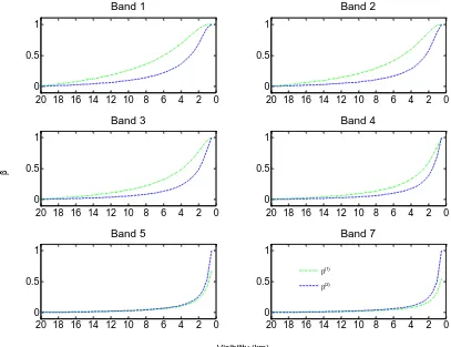
difference between the true signal attenuation and the pure haze weighting, which is more obvious in shorter (i.e. lower-numbered bands) than longer wavelengths (i.e. higher-numbered bands). β V 1

 

is higher than β 2

 

V for shorter wavelengths but this is not the case for longer wavelengths. For shorter wavelengths, β V 1

 

and β 2

 

V show a small difference at longer visibilities. The difference increases as visibility decreases to about 4 km, but then decreases towards 0 km. For longer wavelengths, the difference is only obvious at very short visibilities. At very long visibilities, the difference is not significant, hence use of a single weighting can be considered for these visibilities. Nevertheless, to account for the entire visibilities, the use of different weightings is appropriate due to the inconsistency between the signal attenuation and haze weighting, particularly at moderate and longer visibilities.

Simulation of the Haze Radiance Component, β 2

   

V L 0H

The interaction between solar radiation and the haze constituents affects the spectral measurements made from a satellite remote sensing system and degrades the quality of the images, for example by reducing the contrast between objects and ultimately making them inseparable. Statistically, for a single spectral measurement, haze modifies the mean and standard deviation, but, in a multispectral system the covariance structure of the multispectral measurements is also affected. These effects need to be simulated when using Equation 5 to model haze observed in multispectral Landsat data. We assume that haze can be treated as a random noise that can be modelled as a multivariate Gaussian random variable with mean μ (haze radiance) and covariance matrix C (covariance structure of haze observed by Landsat).

4 Representation of Haze Spatial Properties using Multivariate

Normal Distribution

In simulating haze in remote sensing dataset, we need to take into account its spatial distribution and spectral correlation. In practice, these parameters are difficult to measure due to dynamic behaviour of haze. Here, we assume haze to be spatially uncorrelated, so that it can sensibly simulate haze effects. If the haze was to be spatially correlated, it will appear as patches with high spatial correlation, which are unlikely to represent a real haze condition. Hence, haze can be modelled with an N-dimensional Gaussian probability density function which has the form:

   

N

 

1



 



t ₁

2

2 1

P 2π C exp C

2 

  _ 

 _   _

 

[image:9.595.103.510.147.460.2]

0 2 4 6 8 10 12 14 16 18 20 0 0.5 1 Band 1 0 2 4 6 8 10 12 14 16 18 20 0 0.5 1 Band 2 0 2 4 6 8 10 12 14 16 18 20 0 0.5 1 Band 3 0 2 4 6 8 10 12 14 16 18 20 0 0.5 1 Band 4 0 2 4 6 8 10 12 14 16 18 20 0 0.5 1 Band 5 0 2 4 6 8 10 12 14 16 18 20 0 0.5 1 Band 7 (1) (2) Visibility (km) 

Fig. 3. Plots of  (1) (V) and  (2) (V) against visibility.

where X is an N-dimensional random variable representing the N Landsat bands, i.e. the observed haze, μ _{is the vector of means and} C is the N x N covariance matrix. In order to use this model, we need estimation of μ _and C. We set

 2

   

β V H 0.5

[image:10.595.115.484.195.292.2]

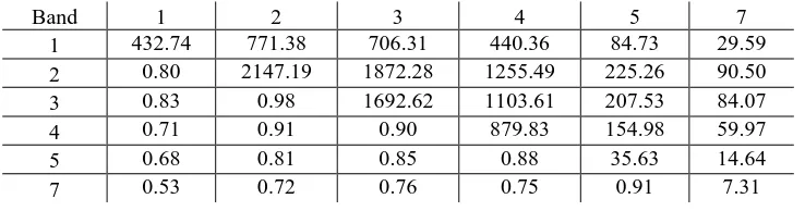
Table 1: Cloud covariances (along and above the diagonal) and correlations (below the diagonal) calculated from Landsat bands 1, 2, 3, 4, 5 and 7.

Band 1 2 3 4 5 7

1 432.74 771.38 706.31 440.36 84.73 29.59 2 0.80 2147.19 1872.28 1255.49 225.26 90.50 3 0.83 0.98 1692.62 1103.61 207.53 84.07 4 0.71 0.91 0.90 879.83 154.98 59.97

5 0.68 0.81 0.85 0.88 35.63 14.64

7 0.53 0.72 0.76 0.75 0.91 7.31

5 Simulation of a Hazy Dataset

The haze component is assumed to be independent of the signal component, so the hazy dataset can be synthesised by adding a weighted pure haze, β 2

   

V L 0.5H to the weighted true signal



1β V L 20 L 1

 



S

 

 O. Here, the true signal component is estimated from Landsat-5 TM dataset (from 11 February 1999 with 20 km visibility, based on the average of 6 stations within 5 to 60 km from the centre of the scene, i.e. Klang Port, Petaling Jaya, Sepang, Serdang, Tanjung Karang and Banting. Based on Equation (16) and for simplicity, we define

 

i S

T L 20 and H_i L_H

 

0.5 . Consequently, due to the vector-based structure of a dataset, the hazy dataset, L V can be written as: i

 

 



 1

 



 2

 

i i i O i i

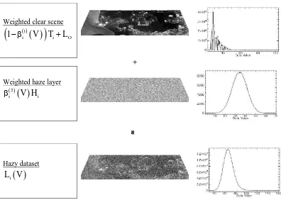
L V  1 V T L + V H ... (20)

Weighted clear scene

 

 



1



i i O

1 V T L

+

Weighted haze layer

 2

 

i V Hi





[image:11.595.95.491.164.446.2]

Hazy dataset

 

i L V

Fig. 4. Process of integrating a hazy layer with a clear data from band 1 to produce a 4 km (V = 4) visibility hazy dataset.

6 Conclusion

In this study, we successfully modelled and simulated haze layers to produced hazy datasets. Spectral and spatial properties of haze are required in order to simulate the haze layers. The spectral properties come from atmospheric path radiance that is simulated using the 6SV1 radiative transfer model. The spatial properties are simulated using 6-dimensional Gaussian probability density function that made use the cloud covariance. The hazy datasets are to be used in studying haze effects on land cover classification in remote sensing data.

References

[1] A. Ahmad and M. Hashim, Determination of haze using NOAA-14 satellite data, Proceedings on The 23rd Asian Conference on Remote Sensing 2002 (ACRS 2002), (2012), in cd.

[2] A. Ahmad and S. Quegan, Analysis of maximum likelihood classification on multispectral data, Applied Mathematical Sciences, 6 (2012), 6425 – 6436.

[3] A. Ahmad and S. Quegan, Analysis of maximum likelihood classification technique on Landsat 5 TM satellite data of tropical land covers, Proceedings of 2012 IEEE International Conference on Control System, Computing and Engineering (ICCSCE2012), (2012), 1 – 6.

http://dx.doi.org/10.1109/iccsce.2012.6487156

[4] A. Ahmad and S. Quegan, Cloud masking for remotely sensed data using spectral and principal components analysis, Engineering, Technology & Applied Science Research (ETASR), 2 (2012), 221 – 225.

[5] A. Ahmad and S. Quegan, Comparative analysis of supervised and unsupervised classification on multispectral data, Applied Mathematical Sciences, 7 (74) (2013), 3681 – 3694.

http://dx.doi.org/10.12988/ams.2013.34214

[6] A. Ahmad and S. Quegan, Haze reduction in remotely sensed data. Applied Mathematical Sciences, 8 (36) (2014), 1755 – 1762.

http://dx.doi.org/10.12988/ams.2014.4289

[7] A. Ahmad and S. Quegan, Multitemporal cloud detection and masking using MODIS data, Applied Mathematical Sciences, 8 (7) (2014), 345 – 353. http://dx.doi.org/10.12988/ams.2014.311619

[8] A. Ahmad, Analysis of Landsat 5 TM data of Malaysian land covers using ISODATA clustering technique, Proceedings of the 2012 IEEE Asia-Pacific Conference on Applied Electromagnetic (APACE 2012), (2012), 92 – 97. http://dx.doi.org/10.1109/apace.2012.6457639

[10] A. Asmala, M. Hashim, M. N. Hashim, M. N. Ayof and A. S. Budi, The use of remote sensing and GIS to estimate Air Quality Index (AQI) Over Peninsular Malaysia, GIS development, (2006), 5pp.

[11] C. Y. Ji, Haze reduction from the visible bands of LANDSAT TM and ETM+ images over a shallow water reef environment, Remote Sensing of Environment, 112 (2008), 1773 – 1783.

http://dx.doi.org/10.1016/j.rse.2007.09.006

[12] E. F. Vermote, D. Tanre, Deuze, M. Herman and J. Morcrette, Second simulation of the satellite signal in the solar spectrum, 6S: An overview, IEEE Transactions on Geoscience and Remote Sensing, 35 (1997), 675 – 686. http://dx.doi.org/10.1109/36.581987

[13] G. D. Moro and L. Halounova, Haze removal for high-resolution satellite data: a case study. International Journal on Remote Sensing, 28 (10) (2007), 2187 – 2205. http://dx.doi.org/10.1080/01431160600928559

[14] M. Hashim, K. D. Kanniah, A. Ahmad, A. W. Rasib, Remote sensing of tropospheric pollutants originating from 1997 forest fire in Southeast Asia, Asian Journal of Geoinformatics 4, 57 – 68.

[15] S. Y. Kotchenova, E. F. Vermote, R. Matarrese and F. J. Klemm Jr., Validation of a vector version of the 6S radiative transfer code for atmospheric correction of satellite data. Part I: Path Radiance, Applied Optics, 45 (26) 2006, 6726 – 6774. http://dx.doi.org/10.1364/ao.45.006762 [16] Y. J. Kaufman and C. Sendra, Algorithm for automatic atmospheric

corrections to visible and near-IR satellite imagery, International Journal on Remote Sensing, 9 (8) (1988), 1357 – 1381.

http://dx.doi.org/10.1080/01431168808954942

[17] Y. J. Kaufman and R. S. Fraser, Different atmospheric effects in remote sensing of uniform and nonuniform surfaces, Advances in Space Research, 2 (5) (1983), 147 – 155. http://dx.doi.org/10.1016/0273-1177(82)90342-8 [18] Y. Zhang, B. Guindon and J. Cihlar, An image transform to characterize and

compensate for spatial variations in thin cloud contamination of Landsat images. Remote Sensing of Environment, 82 (2002), 173 – 187.

http://dx.doi.org/10.1016/s0034-4257(02)00034-2