A PROBLEM IN DATA VARIABILITY ON SPEAKER IDENTIFICATION SYSTEM USING HIDDEN MARKOV MODEL

(1)

Proceedings of the 26th lASTED International Conference ARTIFICIAL INTELLIGENCE AND APPLICATIONS February 11-13, 2008, Innsbruck, Austria

ISBN Hardcopy: 978-0-88986-709-31 CD: 978-0-88986-710-9

A PROBLEM IN DATA VARIABILITY ON SPEAKER IDENTIFICATION

SYSTEM USING HIDDEN MARKOV MODEL

Agus Buono' , Benyamin Kusumoputro"

'Computational Intelligence Research Lab, Dept. of Computer Science, Bogor Agriculture University Dramaga Campus, Bogor-West Java, Indonesia

pudesha@yahoo.co.id

bComputational Intelligence Research Lab, Faculty of Computer Science, University ofIndonesia, Depok Campus, Depok 16424, PO.Box 3442, Jakarta, Indonesia

nynykusumo@yahoo.com

ABSTRACT

The paper addresses a problem on speaker identification system using Hidden Markov Model (HMM) caused by the training data selected far from its distribution centre. Four scenarios for unguided data have been conr'ucted to partition the data into training data andtesting data. The data were recorded from ten speakers. Each speaker uttered 80 times with the same physical (health) condition. The data colIected then pre-processed using Mel-Frequence Cepstrum Coefficients (MFCC) feature extraction method. The four scenarios are based on the distance of each speech to its distribution centre, which is computed using Self Organizing Map (SOM) algorithm. HMM with many number of states (from 3 up to 7) showed that speaker with multi-modals distribution will drop the system accuracy up to 9% from its highest recognition rate, i.e. 100%.

KEYWORDS

Hidden Markov Model, Mel-Frequence Cepstrum Coefficients, Self Organizing Map

1. Introduction

HMM has been widely applied for voice processing with promising results. However voice is a complex magnitude, which is influenced by many factors, i.e. duration, pressure, age, emotion, and sickness [1]. Due to these factors, until now, voice modeling has not reached a perfect result [2].

The research focuses on the problem of HMM application caused by inappropriate training data. Therefore four training data scenarios were proposed to analyze HMM performance, i.e. training data that has distance to its distribution centre: close, far, systematic, and random. The results of this study are expected to be used as the basic for advanced research in voice data modeling using HMM for different kind speaker physical conditions.

2. Speaker Identification

Using HMM

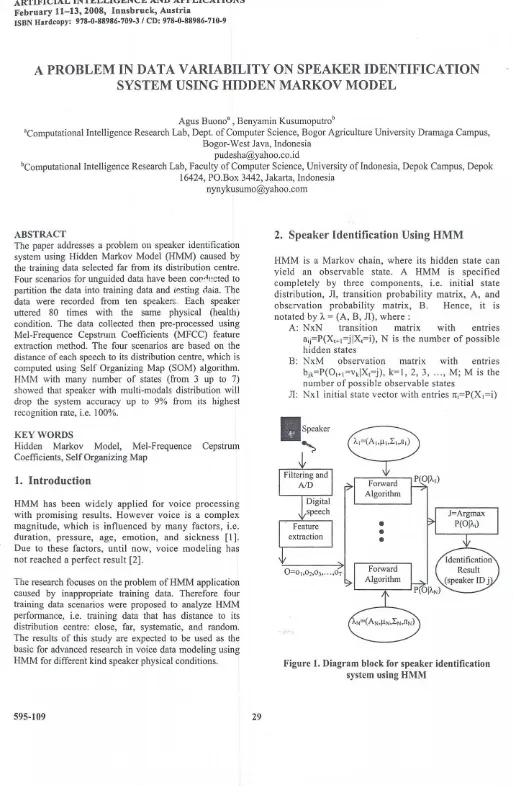
HMM is a Markov chain, where its hidden state can yield an observable state. A HMM is specified completely by three components, i.e. initial state distribution, JI, transition probability matrix, A, and observation probability matrix, B. Hence, it is notated by

zyxwvutsrqponmlkjihgfedcbaZYXWVUTSRQPONMLKJIHGFEDCBA

A= (A, B, JI), where:

A: NxN transition matrix with entries aij=P(Xt+l=jIXt=i), N is the number of possible hidden states

B: NxM observation matrix with entries bjk=P(Ot+l=vkiXt=j), k=l, 2, 3, ... , M; M is the number of possible observable states

[image:1.605.31.545.28.814.2]

JI: Nx 1 initial state vector with entries 1t:i=P(XI=i)

(2)

(

, ,

zyxwvutsrqponmlkjihgfedcbaZYXWVUTSRQPONMLKJIHGFEDCBA

In the Mixture Gaussian HMM, B consists of a mixture parameters, mean vectors and covariance matrixes for each hidden state, C ji, I!ji and L ji, respectively, j=l, 2 , 3 ,

.'" N . Thus value ofb/Ot+l) is formulated as follow:

c

zyxwvutsrqponmlkjihgfedcbaZYXWVUTSRQPONMLKJIHGFEDCBA

b/O /+ ,)

=

LcjiN (O /+ I,fiji'L.j;) i;1

There are three problems in HMM [1], i.e. evaluation problem, P(GlA.), decoding problem, P(QIO, A.), and training problem [3]. Diagram block for speaker identification system using HMM is presented in Figure 1. Probability for each speech data belong to a certain model is computed recursively using forward variable (a)

as illustrated in Figure 2. state

[image:2.599.60.557.95.829.2]

1+t

Figure 2. Illustration of forward variable computation

3.

zyxwvutsrqponmlkjihgfedcbaZYXWVUTSRQPONMLKJIHGFEDCBA

M eth o d o lo g y

3;1-Research Block Diagram

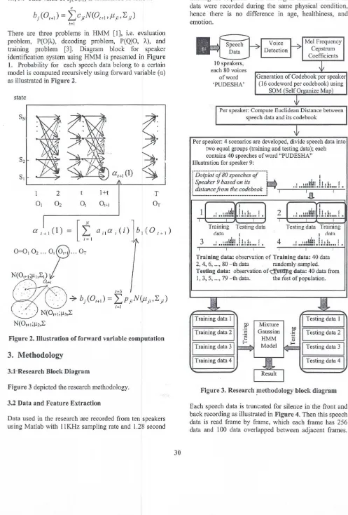
Figure 3 depicted the research methodology. 3.2 Data and Feature Extraction

Data used in the research are recorded from ten speakers using Matlab with 11KHz sampling rate and 1.28 second

duration. Each speaker utters word "PUDESHA" 80 times, which resulted total of 800 speech data. In this case, a speaker has not to follow certain instruction in uttering the required word. Having in mind that these 80 data were recorded during the same physical condition, hence there is no difference in age, healthiness, and emotion.

10speakers, each80voices

of word 'PUDESHA'

Per speaker: Compute Euclidean Distance between speech data and its codebook

Training Testing data

data I

3

"i ••

~~~~~!!.!J.dL.,!

.

Testing data Training

I

zyxwvutsrqponmlkjihgfedcbaZYXWVUTSRQPONMLKJIHGFEDCBA

cilltll

4

II~

""!t~ ~ ~ ~ !!.!J.!:L " "! •

Per speaker:4scenarios are developed, divide speech data into two equal groups (training and testing data); each contains 40 speeches of word "PUDESHA" Illustration for speaker9:

I

!t~~L..

! "

Training data: observationof Training data: 40 data 2, 4, 6, ...,80-th data randomly sampled. Testing data: observationof~g data: 40 data from

1,3,5, ...,79 -th data. the fest of population.

Testing data 11 Testing data

21

Testing data3 1 Testing data

41

Mixture

Training data 4

(3)

On each frame, 20 coefficients of MFCC are computed. Thus, a speech data having T frames will be converted into a T by 20 data matrix. The following Figure 4 depicted the process, [4]. _

Original speech sinyal Signal after removing silence

~-7

Windowing: y,(n) = x,(n)w(n), O:S n :S N-I w(n)=0.54-0.46cos(21tn/(N-l »

'VzyxwvutsrqponmlkjihgfedcbaZYXWVUTSRQPONMLKJIHGFEDCBA

N-J

FFT:

zyxwvutsrqponmlkjihgfedcbaZYXWVUTSRQPONMLKJIHGFEDCBA

X -

L

-2njknl N n - xke

k = O

'¥

Mel Frequency Wrapping: me/if) = 2595*loglO(1+11700)

'V

I

Mel Frequency Cepstrum coefficients~~ Discrete Cosine Transform ~ 20 coefficients

Figure 4. Signal feature extraction using MFCC

3.3 Formulation of Speech Data Variability

Variability indicates how objects positions distributed around its population centre. A population in which its objects scattered close to the centre having less variability as described in Figure 5.

(a) (b)

•

Population

•

~centre~

'.

.

•

• ••

•

zyxwvutsrqponmlkjihgfedcbaZYXWVUTSRQPONMLKJIHGFEDCBA

'.

.

•

• •

•

• •

.'

•

Figure 5. Illustration of population variability (a) higher variability (b) less variability

Using SOM, a codebook consists of 16 codewords from each speaker is generated. The code book representates the centre of population.

~.}o..,": .-.

A distance between a speech data and a certain code book is calculated using the following formula:

d(O, codebook) = ~ average[ 'Ii.d(t, j)]

J=1 tEJ

Where d(tj) is the smallest Euclidean distance between t'h frame and j,h codeword, as illustrated in Figure 6.

0

,

zyxwvutsrqponmlkjihgfedcbaZYXWVUTSRQPONMLKJIHGFEDCBA

7

e

09, Ws

OS

W2 010

03,

,

_e

,

0,

w,e 06 W4

,04

,

e

O2

,

08

W3e

Figure 6: A frame distribution around 5 codewords

,

In this case:

Codebook = (WI, W2, W3, W4, ws), where Wj : j'h codeword

0= 0" O2, 03, ... ,010; where 0,: t'h frame

A distance d(O, codebook) between ° and codebook is:

d(wl ,°3) +d(wl,O 4)

d(O, codebook) = +

2

d(w2,01) +_d(w2,05) +d(w2,06)

+

3

dew 4,°8) +_{dew 4,°10)}

d(w3'O)+ 2 +

dew 5,°7) +_{dew 5,°9)}

2

3.4 Training Data Scenario

For each speaker, its speech data is sorted according to the distance to its population centre in ascending order and divided into two equal groups, i.e. training data and testing data, where each having 40 data. The four scenarios proposed to investigate the system performance are described as follow:

I. Scenario I : first 40 near data to the centre are grouped as training data

2. Scenario 2 : first 40 near data to the centre are grouped as testing data

3. Scenario 3 : 40 training data are sampled "'fO

,,-systematically, i.e. 2, 4, 6, ... , 80 _'h data 4. Scenario 4 : 40 training data are randomly selected.

(4)

Speaker:

zyxwvutsrqponmlkjihgfedcbaZYXWVUTSRQPONMLKJIHGFEDCBA

r l .

. !..!1.t!:!:I:••!..!!.:!:!.._~ ~ _

c

..

.

9 -,----"""-'

-,,··c.=.-==·':T·::"=!~=!~"-'!!-=_...:.!-=J'-!.'-=~'-'~'"""r""'"L"'-"

R -+--_....:!-" ..'-. ""..""h.=!!.!,,-,! ''T.:1,-,~=!-=!:!:= •• ::..:.'''''''--'

'--,.--'--I .'--,.--'--I~'.i

7-,-_--'."'-I'-."".I."'III."'II·TIr.=.~"".""1..z: ,.-_

{j ..:.-"'.!!"'J,::.:i1=!!"'iii=!I!.""!•.:.,:._:..;_=-- _ L.a

5 -.--_--'- ...••••!..•••••••:.".:z:"',t!!.!".'-",,!!.." .,..- __

2 ~ _ _

~.=Ht~wr-

~_

i.ii.li. I

.Il..!.!!!n.!!.!!!!.

5 15 2 5

[image:4.595.48.569.34.806.2]

distance from its codebook

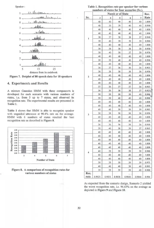
Figure 7. Dotplot of 80 speech data for 10 speakers

4. Experiments

and Results

A mixture Gaussian HMM with three components is

developed for each scenario with various numbers of

states, i.e. from 3 up to 7 states, and observed its

recognition rate. The experimental results are presented in Table l.

Table 1 shows that HMM is able to recognize speaker with unguided utterance at 98.4% rate on the average.

HMM with 6 numbers of states resulted the best

recognition rate as described in Figure 8.

0.99.,---, ~ 0.99

1---~ 0.98

.j---C 0.98

-j---:E

0.98

C 0.981---·

~ 0.98 i:: 0.98 ~ 0.98

0.98

3 4 5 7

Number of State

Figure 8. A comparison of recognition rates for

various numbers of states

Table 1. Recognition rate per speaker for various

numbers of states for four scenarios (Sc.).

Numb er of State Ree.

Se. 3 4 5 6 7 Rate

4 0 4 0 4 0 4 0 4 0 1 . 0 0 0

4 0 3 9 3 9 4 0 4 0 0 . 9 9 0

4 0 4 0 4 0 4 0 4 0 1 . 0 0 0

I 3 8 3 7 3 8 3 8 3 7 0 . 9 4 0

3 9 4 0 3 9 3 9 3 9 0 . 9 8 0

4 0 4 0 4 0 4 0 4 0 1 . 0 0 0

3 8 3 8 3 8 3 8 3 8 0 . 9 5 0

3 9 4 0 3 9 3 7 3 9 0 . 9 7 0

4 0 4 0 4 0 4 0 4 0 1 . 0 0 0

3 9 3 9 4 0 4 0 4 0 0 . 9 9 0

4 0 4 0 4 0 4 0 4 0 1 . 0 0 0

3 6 3 7 3 6 3 6 3 6 0 . 9 0 5

3 8 3 8 3 8 3 8 3 8 0 . 9 5 0

2 4 0 4 0 4 0 4 0 4 0 1 . 0 0 0

4 0 4 0 4 0 4 0 4 0 1 . 0 0 0

3 7 3 6 3 7 3 7 3 6 0 . 9 1 5

3 6 3 6 3 8 3 8 3 7 0 . 9 2 5 ( ~

3 9 3 9 3 9 3 9 4 0 0 . 9 8 9

3 9 3 9 4 0 4 0 4 0 0 . 9 9 0

4 0 4 0 4 0 4 0 4 0 1 . 0 0 0

4 0 4 0 3 9 3 9 3 9 0 . 9 8 5

3 3 8 3 8 3 8 3 8 3 8 0 . 9 5 0

4 0 4 0 4 0 4 0 4 0 1 . 0 0 0

3 6 3 6 3 6 3 8 3 6 0 . 9 1 0

3 9 4 0 3 8 3 9 3 7 0 . 9 6 5

4 0 4 0 4 0 4 0 4 0 1 . 0 0 0

4 4 0 3 9 3 9 3 9 3 9 0 . 9 8 0

4 0 4 0 4 0 4 0 4 0 1 . . 0 0 0

4 0 4 0 4 0 4 0 4 0 1 . 0 0 0

3 9 3 9 3 9 3 9 3 9 0 . 9 7 5

4 0 4 0 4 0 3 9 4 0 0 . 9 9 5

3 9 3 9 3 9 3 9 4 0 0 . 9 8 0

Ree. ~-~ '"

rate 0 . 9 8 2 5 0 . 9 8 3 1 0 . 9 8 3 8 0 . 9 8 5 0 0 . 9 8 4 4 0 . 9 8 4

[image:4.595.72.287.49.341.2]

(5)

Oseen_-1

1 - ._- _{• seen_2}

zyxwvutsrqponmlkjihgfedcbaZYXWVUTSRQPONMLKJIHGFEDCBA

.,

-

I---- - o seen_3

••

0.99

"'

" I-rt

- ~ - =

r-~ I--- I-- Oseen 4

c: 0.98 .' =

-=

- ~

'':: 0.97

,

I-It 1 - _{- ~}

'a

-\ l- I- I- .

.,. 0.96

!'

e

<J

- ~

I--- _{1 -} _{-< l}

.,

0.95

"'

"

0.94

3 4 5 6 7

Number of State

Figure 9. A comparison of recognition rates for

various numbers of states for each scenario

1.00.,---·---= = -.

.fl 0.99

~ 0.99

+---c 0.98 .S: 0.98

:a

0.97

eo 0.97

e

al

0.96

"' 0.96

0.95

4

Training Scenario

Figure 10. A comparison of recognition rates per

scenario

These results indicate that if further objects were sampled for training data then recognition rate will significantly drop.

Distance from its Accuracy:

. codebook Average Scenario 2

•• 11 •

10..,---=-.""! ...:..:!!..:...."'-~!:"-'!:!."-='._=;·.!=!.:!=~!.==._:::.c=--.'= '-_ ':'-'-'--_ 0.99 0.98

9

R +--""~=.._=_=' =..,.'=-=-=.1=.••.=. ''-=--'-' -,--'-- 0.94

••• 1••

zyxwvutsrqponmlkjihgfedcbaZYXWVUTSRQPONMLKJIHGFEDCBA

,Jil.il;l.i.L •.••..

7 1.00

! ::

(j ...!!.!d j!!Hi!i.L ,_ - 1.00

i . .1

5.-_--'-...!--""""~""·:.,i ••"'·I'~!!.2I1'-',,,!!!..I 1--___;-- 0.97 Speaker

.. ~ .. ! .. 0.96 0.93

0.92

1.00

4 -.-_,--,-,-, ...=d.f...,JIM=,i,,,,,,,,lll,,-,, ""---,r--- 0.98

3--'---'-~='-=:=,=:r=--- ..:...'__ -,_ 0.98

2

,-_-=-.

~=:=.,Wr=--" ,--_ 1.00

0.95

0.91

1.00

: i.li. Ii I I

.- __ -'--",.=-" =j.:,!.::::!!::::!!.::::H.!::..:.! !.:!.t --'--_,- __ 1.00 0.99

[image:5.605.49.286.52.670.2]

5 15. 25

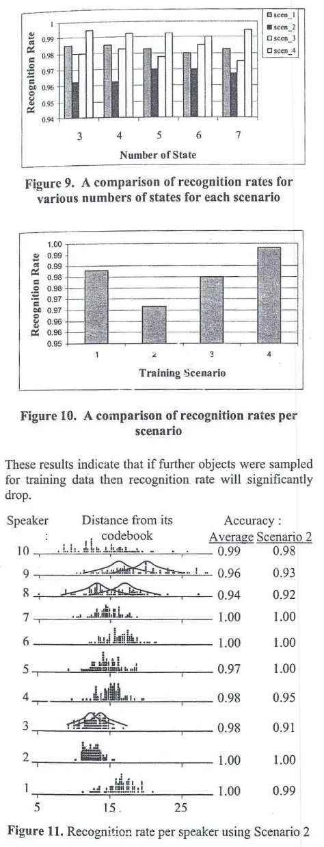
Figure 11. Recognition rate per speaker using Scenario 2

However, this scenario does not affect much HMM

performance to recognize the speaker, i.e. 96.65% is a tolerable rate, due to variability in duration and pressure

has an ignorable effect. In other word, HMM is a robust method to overcome these variations .

Detailed observation in Scenario 2, indicates a

multi-modals speech data distribution of a speaker has a

contribution in lowering the system recognition rate

(Speaker 3,8, and 9) as shown in Figure 11.

These findings predict that the system accuracy will drop further if speaker physical condition (healthiness, age, and

emotion) is different. The prediction is most likely

supported by the fact that a speaker physical condition will affect on the voice distribution pattern.

5. Conclusion

Experimental results proved the robustness of HMM

speaker identification system for unguided utterance

(duration and pressure) by resulting satisfaction

recognition rate (on the average, 96.65% up to 99.3%) using four different scenarios were applied.

The optimal number of states in the HMM is 6 with 98.4% accuracy on the average. Furthermore, sampling

technique in partitioning training and testing data also

affects the system accuracy. In this case, random

sampling gives the best result.

A multi-modals speech data of a speaker will significantly drop the system recognition rate.

6. Future Research

Future research will focused in handling a multi-medals

speech data of a speaker in noisy environment using

modified HMM as classifier. Also, seeks an appropriate

feature extraction to handle the problems, i.e.

multi-modals and noisy data.

References

[1] J. Campbell, "Speaker Recognition: A Tutorial",Proc. of

the IEEE,Vol 85, No.9, 1997, 1437-1462.

[2] L.R. Rabiner, "A Tutorial on Hidden Markov Models

and Selected Applications in Speech Recognition",

Proceeding IEEE, Vol 77 No.2, 1989,257-289.

[3] Rakesh D. "A Tutorial on Hidden Markov Model. Technical Report, Departement of Electrical Engineering, Indian Institute of Technology, Bombay", 1996

[4] Todor D. Ganchev. Speaker Recognition. PhD

Dissertation, Wire Communications Laboratory,

Department of Computer and Electrical Engineering,