49
1
ITB J. Sci. Vol. 42 A No. L 2010, 49-66
Historical Fire Detection of Tropical Forest from NDVI
Time-series Data: Case Study on Jambi, Indonesia
Dyah R. Panuju1, Bambang H. Trisasongko1, Budi Susetyo2, Mahmud A. Raimadoya3 & Brian G. Lees4
IDepartment of Soil Science and Land Resources, Bogor Agricultural University. lalan Meranti. Bogor 16680. Indonesia. Email: [email protected]
2Department of Statistics, Bogor Agricultural University. Bogor 16680. Indonesia. 3Department of Civil and Environmental Engineering, Bogor Agricultural University.
Bogor 16680. Indonesia.
4School of Physical, Environmental and Mathematical Sciences, University of New South Wales at Australian Defence Force Academy. Northcott Drive, Canberra ACT
2600. Australia
Abstract. In addition to forest encroachment, forest fire is a serious problem in Indonesia. Attempts at managing its widespread and frequent occurrence has led to intensive use of remote sensing data. Coarse resolution images have been employed to derive hot spots as an indicator of forest fire. However, most efforts to verify the hot spot data and to verify fire accidents have been restricted to the use of medium or high resolution data. At present, it is difficult to verify solely upon those data due to severe cloud cover and low revisit time. In this paper, we present a method to validate forest fire using NDVI time series data. With the freely available NDVI data from SPOT VEGETATION, we successfully detected changes in time series data which were associated with fire accidents. Keywords: SPOT VEGEl'ATION,' outlier detection: X12-ARIMA.
Introduction
Forest fires in Indonesia have a wide impact on both humans and the environment. Fire accidents are a major cause of loss of life and severe degradation of air quality which, in tum, affect human health [1]. In the case of the islands of Sumatra and Kalimantan, cross-border smoke often raises political problems between Indonesia and Malaysia and Singapore. Fire is also one of the main factors causing environmental degradation. It causes fragmentation of the forest cover leading to greater risk during the subsequent fire episodes. At the global scale, frequent forest fires are one of the major contributors to a change in carbon balance [2] and have become a key component in climate change .
. Efforts to combat forest fire are underway. A special task force to deal with forest fire has been assembled. In a number of major crises, it has been assisted
50
Dyah R. Panuju, et al.by ASEAN fire fighters to reduce the trans-national impact. With very extensive Whi areas affected, remote sensing provides invaluable data for both decision also makers and local fire fighters. Remote sensing also offers continuous info
monitoring for tactical decision making [3]. prac
sho' Fire frequently occurs in both tropical and boreal forests. In boreal forests, uset several episodes of large forest fires have been recorded which have raised the drar importance of time-series assessments [4]. In tropical forests, major forest fires cou: have been associated with the EI Nino Southern Oscillation (ENSO) which is dat;; associated with extreme drought making them regional, rather than local,
Ob\ phenomena [5]. It was also worsened by human activity encroached not only to
primary forest but also preserved forest that can lead to carbon leaks from ND tropical area. Indeed, to detect and prove tropical forest encroachments, ApI particularly if triggered by fire, are difficult due to frequent precipitation which veg' inhibits fire. Monitoring by remote sensing has been difficult because of limited No!
revisit time of high resolution sensors. Although many hot spot data have been Enn produced by many satellites, but it has been limitedly proven as real fire spot. ana As fire is very dynamic, time series data are required to comprehensively assess han the progress of the phenomenon. Coarse resolution remote sensing data offer Rec possibilities to provide time-series data over extensive areas. [16
Time-series remotely sensed data have been used in other applications. In Ext meteorology, Liu et at. [6] presented a method to map evapotranspiration using det. time-series data. In agriculture, using the A VHRR sensor, Schwartz et al. [7] We
demonstrated the capability of remote sensing data to derive information on the frOJ start of the spring growing season to quantify the influence of climate change. Ins1 Another study, Julien et at. [8], emphasized the importance of long time-series dat remote sensing data to assess the contribution of volcanic aerosols to the dat, vegetation dynamics of the European continent. Because of the return
frequency, Moderate Resolution Imaging Spectrometer (MODIS) data has been
2
preferred for many of these land-based remote sensing applications such asforest phenology [9,10]. Tir
cor In the case of forest fire, time-series data have been employed for various mu purposes. Mapping of the burned scar has been the most common application. mu Coarse remotely sensed images have been used for this purpose including both sig NOAA AVHRR and MODIS [11]. Generally, forest fire has been assessed the through time-series composite techniques. This minimises radiometric problems
51
Historical Fire Detection from NDVI Time Series Data
While previous efforts have concentrated on mapping fire-affected areas, it is
vc
on also important to determine the time of the accident. In Indonesia, this information is important for law enforcement as massive slash-and-burn
us
practices are illegal, in particular for plantation companies. Goetz et al. [13]
showed NDVI patterns of burned and unburned areas which were particularly
ts, useful for studying post-burn recovery. According to their report, fire had a
he dramatic effect in the NDVI time series data, suggesting that the technique 'es could be used to confirm the time of fire initiation, especially from hot spot
IS data.
ai,
Obviously, the NDVI is not a perfect choice to the problem. Viovy [14] showed
[0
)In NDVI dependencies on atmospheric disturbances due to volcanic eruption.
Its, Application of NDVI on forage prediction was also found limited. Other
eh vegetation indices have been invented and showed better performance [15]. ed Nonetheless, applying those newly-developed vegetation indices such as :en Enhanced Vegetation Index (EVI) designed from MODIS data in time series
at. analyses is usually limited due to availability of the dataset itself. On the other :ss hand, NDVI provides long-term data capture suitable for time series analyses. fer Recent reports still have commented the usefulness of NDVI time series data
[16,17].
Extending the work of Goetz et al. [13], and to evaluate the quantitative determination of fire initiation, we carried out an analysis of time series data. We employed the X12-ARIMA algorithm to provide the date automatically from the NDVI data of SPOT VEGETATION made available by Vlaamse Instelling voor Technologisch Onderzoek (VITO). The use of freely available data is a significant benefit for the preliminary screening for higher resolution data capture for operational purposes.
urn
セ」ョ@
2 Time Series Analysis as
Time series data area chain of observations acquired over time and often contain a constant time lag. The observations can be single variable or OllS multi variable which, in remote sensing terminology, corresponds to single and on. multiple data respectively. The data are not limited to raw electromagnetic 'oth signals, but also cover derivative information such as spectral indices or
sed thematic data.
;!1lS
52
Dyoh R. Ponuju, et01.
Unfortunately, the stationary condition occurs rarely and therefore a XI2-A differencing technique is often used to handle non stationary series. Chen, (AO), I
"-Common modelling on single variable time series has exploited the of outll Autoregressive Moving Average (ARMA) or the Autoregressive Integrated contaill Moving Average (ARIMA) modelling philosophies introduced by Box and ウエッ」ィ。セ@ Jenkins [19]. While the ARIMA is useful for assessing time series data, it fitted 11 suffers from the effects of seasonality which is naturally found in many the sta circumstances. In order to accommodate this, the X procedure has been used as Chen a an alternative procedure for seasonal adjustment.
In the ( The combination (XII-ARIMA) has been introduced to compensate for the lack of mull of an explicit model functional to the series and to minimise the unsmoothed locatiol first and last observation of the series [20]. Later, the model was updated to canopy X12-ARIMA by Findley et al. [21]. Following the Box-Jenkins notation, a Hence, seasonality-induced ARIMA model is represented as (p,d,q)(P,D,Q). Notations
p and P point to the ordinary and seasonal autoregressive respectively, while q and Q indicate the properties of moving averages. Respectively, d and D specify ordinary and seasonal differences in from the primary series. The use of XII-ARIMA, the previous version of seasonal XII-ARIMA, in environmental research
with th was found, such as on climate research [22].
3
Outlier DetectionOutlier detection was an improvement capacity of ARIMA to deal with
outrageous evidences during the series. Adya et al. [23] defined outliers or where contaminant data as unusual observations that shift from the general pattern of
the set. While time series data generally contain outliers, they have been 9(B) ::::( disregarded in many studies. There are only a few which identify the various
presem types of outlier. Fox [24] noted two types of outlier, namely type I and type II.
otherw: Type I relates t9 .the state where a single observation can be influenced by gross
presum error. Another type is used when the influence is observed not only on a specific 2
(Ja • observation, but continues onto the succeeding observation. Later, type I and
type II were identified by Chang et ai. [25J as additive (AO), and innovational
Taken
(10), outliers respectively. If a series is under consideration, a single
estimat observation in the series can be either AO, 10 or neither. Iterative procedures to
test for the presence of outliers have been presented [25-27J under the ARIMA framework. In addition to these types of outlier, Tsay [26] presented the level shift (LS), which was then divided into the level change (LC) or permanent change (PC) and transient change (TC) outliers. The most recent paper by
where! Kaiser and Maravall [28] estabHshed another type of outlier namely the
observ, seasonal level shift (SLS).
Historical Fire Detection from NDVI Time Series Data 53
=fore a X12-ARIMA automodelling can assess the four types of outliers discussed by Chen and Liu [29], namely the innovational outlier (10), the additive outlier -(AO), the transient change (TC) and the level shift (LS). To detect the presence ted the of outliers in time series data, the residual of the series is determined. Residuals tegrated contain data unexplained by the model. The assumption of the time series
lox and stochastic model is the homogeneity of variance and stationarity of data. The data. it fitted model is evaluated by computing the minimum mean square error, while 1 many the stationarity is.r evaluated from the pattern of the corresponding residuals.
used as Chen and Liu [29] presented equations to compute residuals for the outliers.
In the case of forest fire hot spots, the model should accommodate the detection the lack of multiple outliers. This is due to the high probability of re-burn in the same 100thed location related to time lag between estate preparation (land clearing) and lated to canopy closing. Time lag could be a year in case of timber plantation [30]. ltion. a Hence, the ARMA process can be represented as follows
)tations while q
'" m 9(B)
specify Y =
L
co.L.(B)lt(L)+ a (1)t j
=
I J J J cp(B)a(B) t )f X11esearch
with the error forecast as
(2)
11 with
tiers or where 9, a, cp are polynomials of B; cp(B) = ICPI (B) ... cpp (B)P and
ttern of
e been 9(B)=(l9 B ... 9 BP)are stationary; and I,(tj) serves as indicator for the
1 p
various
type II. presence of outliers and is a binary number where equals to 0 if t f:. t\ and 1
otherwise. co represents amount and pattern of outlier respectively, while al is
y gross
:pecific presumed to be a sequence of independent variable with mean 0 and variance
2 Oa • セ@ I and
ational
Taken into account the seasonal pattern of the data, the XI2ARIMA [21] single
ures to estimates regression ARIMA models of order (p,d,q)(P,D,Q) for YI as
.RIMA e level
q> (B)<I>p(Bs)(lB)d(lBS)D(y
f
Pi
Xit)=6 (B)E>Q(Bs)a (3)nanent p t i=l q t
per by
where s is the length of seasonal period; s=12 represents 12 month of an annual
Iy the
54 Dyoh R. Ponuju, et 01.
(jlP(z),<DP (z),eq (z),eQ (z) with degrees of p, P, q, Q respectively have a
constant term equal to 1.
4
Methodology
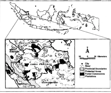
The research was carried out around the Berbak National Park in eastern wetland of lambi province, one of three Ramsar reserves in Indonesia (Figure
I), The area has suffered from logging and frequent fires for land clearing,
particularly in the dry season [31
J.
It
A
• City
セ River
c:J Provincial Boundaries I8TI Protected Areas _ Forest Concessions
[image:6.614.134.489.355.654.2]D Plantations
Figure 1 Site location. Dark and light polygons represent forest concessions
and plantations respectively. The Berbak NP is located on eastern coastal region.
The study made use of both medium and coarse remote sensing data. Landsat ETM, as medium resolution data, provided actual fire data. We selected a Landsat ETM scene of lambi (path/row 125061) acquired on 1 September 1999 which showed a large active fire. It is difficult to have fire evidence data and to capture actual fire in tropical region on image (such as Landsat ETM)
due ref
dw Inc COl fro
Se ne' Th tra USt co;
Us
art an. Th
tlu
be sy:
sel 19 ag lia ca
W
tセ@
an ap int me idi dil au
leI
thc
Wt
55 Historical Fire Detection from NDVI Time Series Data
due to cloud cover, therefore the data was a valuable evidence of fire for a
e a reference on further analysis. No radiometric adjustment was applied, mainly
due to the laGk of meteorological data. Hotspot data collected from the Indonesian Institute of Space and Aeronautics was also employed for completing and cross checking the evidence. The hotspot data were produced from NOAAAVHRR from some platforms including NOAAI2, 15 and 16. Several techniques for bum scar delineation can be found in the literature, ern
nevertheless we found a paper by Koutsias et al. [32] particularly interesting. ure
The paper discussed the application of the IntensityHueSaturation ng,
transformation on specific colour composite image. The technique proved useful, taking advantage of the fast computation of intensity, hue and saturation components from a redgreenblue image composite.
Using the fire extent derived from the medium resolution image, the burned area was gridded to obtain several samples as the main locations for time series analysis. We used NDVI data of SPOT VEGETATION from the VITO website. The NDVI data were distributed as 1Oday composite images, hence there were three for each month and the first NDVI (NDVI\) data represented a time span
between day 1 and day 10, NDVI2 denoted day 11 to day 20, and NDVI3
symbolized day 21 to day 30 of the month. To ease extraction of the NDVI time series at each sample point, we stacked all NDVI data taken between 1 April 1998 and 21 February 2005. Due to the limits of the ARIMA model, a monthly aggregation was carried out. To do this we selected the approaches presented by
Jia et at. [33]. The monthly average (MA) and monthly peak (MP) were
calculated using following equations.
MANDV1 = mean(NDVlh NDVlz, NDVI3) (4)
MPNDV1 = max(NDVIh NDVJz, NDVh)
(5)
56 Dyoh R. Ponuju, et 01.
various remote sensing data sources, we also considered hotspots around the site at a distance of 0.02 degree.
5
Results and Discussion
5.1
Fire delineation from Landsat ETM data
The IRS transform is a simple image transformation which has been used for many applications including multiresolution data fusion and enhancement of terrain for interpretation. While those applications require a twoway transformation (ROB to IHS and back to ROB), the thematic extraction of
Koutsias et al. [32] only requires a forward transform. Dealing with
multi-spectral images such as Landsat, the key step to extract bum scars is to find suitable band combinations. Koutsias et ai. [32] suggested bands of 7, 4, and 1 for the best discrimination. In this study, we used that suggested combination and compared it to
a
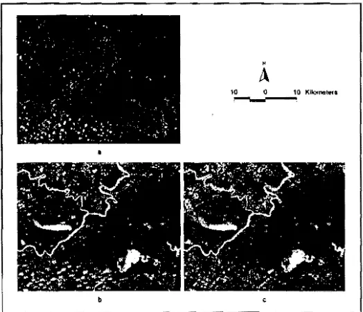
combination of 7-4-2. Figure 2 presents a Landsat colour composite (ROB 542) and the hue components after the IRS transform. The Landsat image coincidentally captured a large active fire along with associated smoke. The burnt area is located in the centre of the image surrounded by various land use types including fragmented forests, clear cut and agricultural fields (Figure 2a).Fr sh
in
o
fiI W In su co bu direo
co of he
Ai
5..
Tl au an in m( no Fi; sel inl
inl de Ea pa co ha ex int
aU!
sel anI Figure 2 Colour composite image (a) in comparison with hue components of
[image:8.614.185.447.480.705.2]Historical Fire Detection from NDVI Time Series Data
57
,und the From the composite image, the area apparently was burned several times over a
short period of time. Slightly different levels of reddish are shown which indicate different intensities of burning or different times of slashandburn. Considering that frequent downpours in the eastern Jambi provinces can inhibit fire spread, it can be estimated that attempts to bum started before August 1999. We noticed a good agreement between visual analysis and derived hue images. In general both hue images present clear discrimination of the bum scar and its
Ised for surrounding land cover. Nonetheless, the hue component derived from 742
nent of composite is shown in slightly lower contrast (Figure 2c). In the image, both
\Noway burned area and bare soil are presented in a similar tone, which leads to
:tion of difficulty in the automated delineation of the burned surface. In general, our
I multi result was in agreement with the conclusion of Koutsias et al. [32] that a
to find combination of 741 produced a better discrimination than of 742. The result
l, and 1 of IHS transform was used to delineate bum area which covered about 1342
)ination hectares. The area was then gridded and we obtained 20 sample series for X12
. colour ARIMA modelling .
n. The
ociated
5.2
ARIMA Automodeling of Tropical Forest
ded by The seasonal adjustment automodelling was set up for selecting, in order, the
:ultural autoregressive, differencing, and moving average respectively both on ordinary
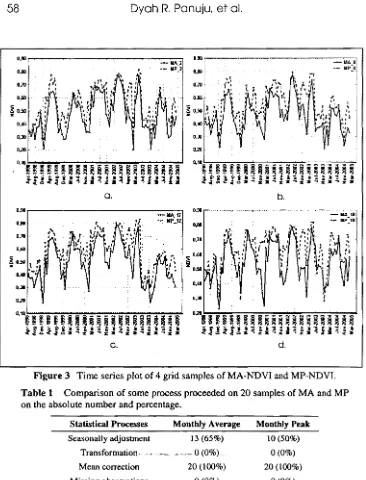
and seasonal series of data [34]. The model used was the economic application in which Easter and trading day components were taken into account. This model had to be adapted to remove those unnecessary components as they had no meaningful relationship to vegetation greenness represented by NDVI. Figure 3 shows time series data of 20 grid samples. The figure illustrates time series pattern of NDVI which affected by seasonality and therefore difficult to interpret. Visual interpretation solely based on these series might mislead information retrieval if the seasonality is present. Statistical tests such as outlier detection could make a clarification for the problem.
Each sample can be modelled on a particular ARIMA model. Instead of using a particular madeJ,. we us.ed.automQdel ARIMA to allow us more focus on the comparison of NDVI data representation of MA and MP. A particular model has significant meaning in forecasting and it is beyond the scope of this study to explain the difference on each series due to the limitations of our ground information. Models of the 20samples varied in almost all order of autoregressive, differencing and moving average for both ordinary and seasonal series. Comparisons of the performance of the automodelling processes of MA and MP are presented in Table 1.
58
Dyoh R. Ponuju, et 01. sample waspn sample identifi sample ヲッイ・」。セ@ andM reliable [13]ru here tt of ext o. Diffen specifi aggreg from セ@ reliabl Partic have 1 been repeal intern surfa( remofc.
Figure 3 Time series plot of 4 grid samples of MANDVI and MPNDVLTable 1 Comparison of some process proceeded on 20 samples of MA and MP Detee
on the absolute number and percentage. occur
dセセMMMMMMセセMMMMMMMMMMM⦅セセセX@
- - MP)
PNQPセ@
, •i , i
セ@ セ@セ@ セ@ セ@ セ@
ijセ@セ@ セ@ セ@
ijセ@セ@ セ@ セ@
iゥャAゥャAZセャZセャZセャZセZZセZZ@ b. O.lll 0,11 . O,QI d. Statistical Processes Seasonally adjustment Transformation , .... Mean correction Missing observations Seasonality "significant" Forecasting error> 10% Monthly Average 13 (65%) セNLNM 0 (0%). 20 (100%) 0(0%) 2.0 (loo%) 6 (30%) condi Monthly Peak sharp 10 (50%) [35],
0(0%) ass un
20 (100%) annUl
0(0%) data
11 (55%) preci
8 (40%) there
オウゥョセ@
Table 1 shows similar performances between MA and MP on some processes,
The particularly in the requirement of data transformation, mean correction and
dete( detection of missing observations for the samples .. A significant difference of
took MA and MP was shown in the detection of the seasonality effect on each
sample series. All MA series had a significant seasonal pattern while only II we a
L
59
i@
, "
'. ! 1
セ
I,セー@
)cesses, on and encc of
1I1 each
)l1ly II
Historical Fire Detection from NDVI Time Series Data
samples (55%) of MP series were affected by seasonality. However, seasonality was probably present in the remaining samples of MP. Most of the MA and MP samples were seasonally adjusted allowing proper seasonal pattern identification. All MA samples were seasonally significant which means that all
samples were seasonally affected. Another process shown in Table 1 is
forecasting error. Slight differences in performance were shown between MA and MP which indicated that 6 samples of MA and 8 samples of MP were not reliable for quantitative analysis. It appears that previous studies by Goetz et ai. [13] assumed equal significance of series taken from different sites. It shown here that even if all samples were taken from a similar condition (delimitation of extracted burned areas), different characteristics of series were evident. Different aggregation processes by assigning average or maximum values over specific time frame produced different results. We observed that excessive aggregation would likely generate biased interpretation. Using information from Table 1, we were able to show those differences and hence able to select reliable series.
5.3
Outlier ExtractionParticularly on the eastern provinces of Sumatra, slashand burn techniques have been practiced for land clearing. Hence, a high number of forest fires have been detected in this region. Due to the humid climate and high rainfall, repeated burning has been observed as slashandburn activities may be interrupted by the rain. Burning can be continued several days later once the surface has dried. This pattern creates a high frequency of hot spots detected by remote sensing and explains why hot spots occur at the same location.
Detection of forest fire using Landsat data indicated that repeated burning occurred on the test site. Theoretically, the fire created a hiatus in vegetation condition represented on the NDVI time series data where the NDVI values sharply decreased. Since long term observations can contain seasonal patterns
[351, that ーィ・ョYャdセtャoョ@ shoulli beilccounted for during data processing. We
assumed that tenday NDVI or their monthly aggregation data were shown as an annual repeated pattern. Hence outlier detection looked for any hiatus in the data while taking account of the seasonal pattern. The outlier detection offers precise identification of date (or in our case month and year) of fire occurrence, therefore improves on Goetz et ai. [l3} findings. Results of outlier detection using MA and MP are presented in Table 2.
60
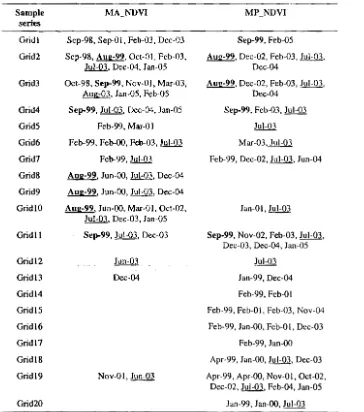
Dyoh R. Ponuju, et 01.the site. There appears to be little difference in performance between MA and MP on outlier detection. Many outliers were successfully detected on MA and MP samples. Some were shown to share an identical date with our hot spot database and the Landsat image. We considered a month after outlier date to be identical because the change of greenness due to fire can be detected after the burning. particularly if it was taken place on last ten day of the month.
Table 2 Outlier detection using monthly average and monthly peak data. Outliers in bold indicate in agreement with Landsat image, while in underline in agreement with hot spot data respectively.
Sample
series
Grid 1 Sep98, SepOl, Feb03, Dec03 Sep99, Feb05
Grid2 Sep98, Aug99, OctOl, Feb03, Aug99, Dec02, Feb03,l!!l::Q.l, lul03, Dec04, lan05 Dec04
Grid3 Oct98, Sep99, NovOl, Mar03, Aug99, Dec02, Feb03, Jul03, A.Ygjll, Jan05, Feb05 Dec04
Grid4 Sep99,lul03,Dec04,Jan05 s・ーMYYLf・「セSLjオャMPS@
GridS Feb99, MarOI l!!l::Q.l
Grid6 Feb99, FebOO, Feb03, Jul03 Mar03,lY.!JU
Grid7 Feb99, Jul03 Feb99, Dec02, Jul03, Jun04
GridS Aug99, lunOO, JuI03, Dec04
Grid9 Aug99, JunOO, Jul03, Dec04
Grid 10 Aug99, lunOO, MarOI, Oct02, JanO I, Jul03 Jul03, Dec03, Jan05
Grid 1 1 Sep99, Jul03, Dec03 Sep99, Nov02, Feb03, Jul03, Dec03, Dec04, JanOS
Grid 12 Jun03 Jul03
Grid 13 Dec04 Jan99, Dec04
GridI4 Feb99, FebOl
GridI5 Feb99, FebOl, Feb03, Nov04
Grid 16 Feb99, JanOO, FebO i, DecOJ
GridI7 Feb99, JanOO
GridlS Apr99, JanOO. Jul03, Dec03
GridI9 NovOi, Jun03 Apr99, AprOO, NovOl, OcI02. Dec02, Jul03, Feb04, Jan05
Grid20 Jan99, JanOO, Jul03
T
w
A
pI cl a1
c(
sa w
a(
pI
Tl
bt th [3 pa of 01:
w:
01: co
[image:13.614.145.509.332.744.2]61 Historical Fire Detection from NDVI Time Series Data
j
j
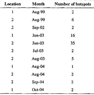
The result shows that the MA and MP contained four series with outliers which were detected coincident with fire detection from Landsat image on August/September 1999 at different sites (Grid 2, 3,4 and 11). Based on the presumption that significant effect of fire would be manifested on outrageous change on NDVI series, it could be inferred that the corresponding sample was affected by fire. In addition, we obtained seven samples of MA and MP that contained similar dates to detected hot spots (July 2003). There were fifteen samples of MA and fourteen samples of MP which showed good agreement with hotspot data, although these could not be validated due to the lack of additional reference data. Complete hotspots detected in samples area are presented in Table 3.
Table 3 Number of hospots on sample areas (locationI) or ± 0.02 degree of longitude or latitude (location2), and their date (monthyear).
Location Month Number of hotspots
Aug99 2
2 Aug99 6
2 Sep02 2
Iun03 16
2 lun03 35
2 lul03 2
2 Aug03 5
Aug04
2 Aug04 2
2 Sep04 2
OcI04 2
[image:14.614.206.404.406.606.2]62 Dyoh R. Ponuju, et 01.
MP comprised 6 outliers in TCtype and 7 in LStype was also coincident with hotspot of July 2003 in surrounding site or with a month later of hotspot detected in the site. We did not deal with all types of outliers due to limitations of information to deliver proper explanations.
The result of outlier detection of MA and MP were quite different, however they showed that both achieved their aim. Many outliers could not be precisely linked to burning activity on the corresponding date of hotspot. Some other possible activities, such as logging. can affect a similar change of vegetation greenness. It appears that outlier detection of NDVI series is a potential method to explore historical evidences of vegetative area. Outliers could be a sign that there was an important phenomenon occurred on the specific date. Detailed information should be explored to prove and dig up initial information provided from outlier detection analysis.
6
ConclusionsIn this paper, the application of out1ier detection using XI2ARIMA for exploring historical evidence of forest fire was investigated. It seems that part . of lambi natural forest have been suffering from encroachment since before August 1999 and sti11 continuing. Using illS transformation, hue image of bands 741 composite could discriminate clearly bum scars. Mapping of bum scars confirmed active fire encroaching the test site. Image extraction on sample area provided information on the efforts to convert natural forests to cultivated area. Using XI2ARIMA the efforts were detected as outliers on NDVI time series. LANDSAT ETM acquisition date was identified in the outlier list. Four outliers were detected on MA and two on MP samples which coincide with hotspots data and LANDSAT image. In addition, three MA and three MP samples were able to detect outliers which correspond with a month after fire captured on image. Apparently, sensitivity on outlier detection using MA and MP showed indifferent. Using automodelling of ARIMA, we showed a quantitative analysis of selected sites. We extended the approach outlined by Goetz et al. [13J by providing the date of the events from time series databases of NDVL Research of Goetz et al. [13J tent to disregard this selection and generally assumed that all sample sets are equally reliable.
Despite recent avai1ability of many vegetation indices, the NDVI time series data were shown useful, mainly due to their longterm accessibility. Nonetheless, we urge further assessments to exploit other indices such as the Enhanced Vegetation Index (EVI). Comparison of the use of different vegetation indices may provide a more reliable index for detection of historical
changes in vegetated areas. Vegetation indices of MODIS (Moderate
Historical Fire Detection from NDVI Time Series Data 63
with understanding due to its detailed scale. Improving capacity on ARIMA
Itspot modelling in analysing ten days data would also enhance precision in outlier
ltions detection.
Acknowledgements
vever We would like to thank VITO, Belgium for their support obtaining SPOT
:isely VEGETATION dataset and BPPSDIKTI, Indonesian Ministry of Education for
other the scholarship. Part of the references was obtained from the Library of
arion Universita degli Studi di Roma Tor Vergata and we are grateful for Profs.
:thod Domenico Solimini and Leila Guirerro assistances.
I that
ailed
,ided
7
References
[1] Mott, J.A., Mannino, D.M., Alverson, CJ., Kiyu, A., Hashim, J., Lee, T.,
Falter, K. & Redd, S.C., Cardiorespiratory Hospitalizations Associated
with Smoke Exposure during the 1997 Southeast Asian Forest Fire, International Journal of Hygiene and Environmental Health, 208, 7585, , for
2005 . . part
:!fore [2] Harden, l.W., Trumbore, S.E., Stocks, BJ., Hirsch, A., O'Neill, K.P. &
セ・@ of Kasischke, E.S., The Role of Fire in the Boreal Carbon Budget, Global
burn Change Biology, 6 (Supp 1), 174184,2000.
n on [3] Keramitsoglou, I., Kiranoudis, C.T., Sarimveis, H., Sifakis, N., A
ts to Multidiscplinary Decision Support System Jor Forest Fire Crisis
's on Management, Environmental Management, 33, 212225, 2004.
I the [4] Arniro, B.D., Orchansky, A.L., Barr, A.G., Black, T.A., Chambers, S.D.,
Ihich Chapin III, F.S., Goulden, M.L., Litvak, M., Liu, H.P., McCaughey, J.H.,
. and McMillan, A. & Randerson, J.T., The Effect of Post-Fire Stand Age on
ionth The Boreal Forest Energy Balance, Agricultural and Forest Meteorology,
lSlng 140,4150,2006.
)wed
[5] Fuller, D.O. & Murphy, K. The ENSO-Fire Dynamic in Insular Southeast
d by
Asia, Climatic Change, 74, 435455, 2006. lases
[6] Liu, J., Chen, J:M: & Cihlar, J., Mapping Evapotranspiration Based on
and
Remote Sensing: An Application to Canada's Landmass, Water Resource Research, 39, doi: 1O.1029/2002WRooI680, 2003.
cncs [7] Schwartz, M.D., Reed, B.C. & White, M.A., Assesing Satellite-Derived
i lity. Start-oJ-Season Measures in The Conterminous USA, International
, the Journal of Climate, 22, 17931805,2002.
:rcnt [8] Julien, Y., Sobrino, J.A. & Verhoef, W., Changes in Land Surface
rical
,
,
Temperatures and NDV! Values Over Europe Between 1982 and 1999,:;rate Remote Sensing of Environment, 103, 4355, 2006.
etlcr
I
64
Dyoh R. Ponuju, et01.
[9] Ahl, D.E., Gower, S.T., Burrows, S.N., Shabanov, N.V., Myneni, RB. &
Knyazikhin, Y, Monitoring Spring Canopy Phenology of A Deciduous
Broadleaf Forest Using MODIS, Remote Sensing of Environment, 104, 8895, 2006.
[10] Xiao, X., Hagen, S., Zhang, Q., Keller, M., Moore III, B., Detecting
Phenology of Seasonally Moist Tropical Forests in South America with Multi-Temporal MODIS Images, Remote Sensing of Environment, 103, 465473, 2006.
[11] Chuvieco, E., Ventura, G., Martin, M.P. & Gomez,!., Assessment of
Multitemporal Compositing Techniques of MODIS and A VHRR Images for Burned Land Mapping, Remote Sensing of Environment, 94, 450
462,2005.
[12] Holben, B.N., Characteristics of Maximum-Value Composite Images
from Temporal AVHRR Data, International Journal of Remote Sensing, 7, 14171434, 1986.
[13] Goetz, S.1., Fiske, G.1. & Bunn, A.G., Using Satellite Time-Series Data
Sets to Analyze Fire Disturbance and Forest Recovery Across Canada,
Remote Sensing of Environment, 101, 352365, 2006.
[14] Viovy, N., Automatic Classification of Time Series (ACTS): A New
Clustering Methodfor Remote Sensing Time Series, International Journal
of Remote Sensing, 21, 15371560,2000.
[15] Moleele, N., Ringrose, S., Amberg, W., Lunden, B. & Vanderpost, c.,
Assessment of Vegetation Indexes Usefulfor Browse (Forage) Prediction In Semi-Arid Rangelands, International Journal of Remote Sensing, 22, 741756,2001.
[16] Bradley, B.A., Jacob, RW., Hermance, J.F. & Mustard, J.F., A Curve
Fitting Procedure to Derive Inter-Annual Phenologies from Time Series of Noisy Satellite NDVI Data, Remote Sensing of Environment, 106, 137
145,2007.
[17] Busetto, L., Meroni, M. & Colombo, R, Combining Medium and Coarse
Spatial Resolution Satellite Data to Improve The Estimation of Sub-Pixel NDVI Time Series, Remote Sensing of Environment, 112, 118131, 2008.
[18] Wei, W.W.S., Time Series Analysis: Univariate and Multivariate
Methods, Pearson/AddisonWesley, Boston, 2006.
[19] Box, G.E.P. & Jenkins, G.M., Time Series Analysis: Forecasting and
Control, HoldenDay, San Francisco, 1976.
[20] Dagum, E.B., The X-ll-ARIMA Seasonal Adjustment Method, Statistics
Canada, 1980.
[21] Findley, D.F., Monsell, B.c., Bell, W.R, Otto, M.e. & Chen, BC., New
Capabilities and Methods of the X-12-ARIMA Seasonal-Adjustment
[2
[2
[2
[2
{セ@
{セ@
[:
65 Historical Fire Detection from I\lDVI Time Series Data
Program, Journal of Business and Economic Statistics, 16, 127152, ,R.B.&
1998.
セ」ゥ、オッオウ@
[22] Pezzulli, S., Stephenson, B. & Hannachi, A., The Variability of
セョエL@ 104,
Seasonality, Journal of Climate, 18,7188,2005.
[23] Adya, M., Collopy, F., Armstrong, J.S. & Kennedy, M., Automatic
'etecting
Identification of Time Series Features for Rule-Based Forecasting, ica with
International Journal of Forecasting, 17, 143157,2001. nt, 103,
[24] Fox, AJ., Outliers in Time Series, Journal of Royal Statistical Society
Series B, 34, 350363, 1972. men! of
Images [25] Chang, I., Tiao, G.c. & Chen, C., Estimation of Time Series Parameters
14, 450 in The Presence of Outliers, Technometrics, 30, 193204, 1988.
[26] Tsay, RS., Outliers, Level Shifts and Variance Changes in Time Series,
Images Journal of Forecasting, 7,120,1988.
Ising, 7, [27] Chen, C. & Liu, L.M., Joint Estimation of Model Parameters and Outlier
Effects in Time Series, Journal of American Statistical Association, 88, 284297, 1993a.
'!s Data
セ。ョ。、。L@ [28] Kaiser, R & Maravall, A., Seasonal Outliers in Time Series, Banco de Espana, Madrid, Spain, 2001.
A New [29] Chen, C. & Liu, L.M., Forecasting Time Series with Outliers, Journal of
Journal Forecasting, 12, 1335, 1993b.
[30] Lorenzo, E.P. & Munoz, c.P., Land Clearing without Fire: A Model for
ost, c., Preparing Timber Plantation Development in Indonesia, in Proceeding of
セ、ゥ」エゥッョ@ Workshop on Peatland fire in Sumatera: problems and solutions,
ng,22, Palembang, 1011 December 2003.
[31] Stolle, F., Chomitz, K.M., Lambin, E.F. & Tomich, T.P., Land Use and
Curve Vegetation Fires in Jambi Province, Sumatera, Indonesia, Forest Ecology
, Series and Management, 179,277-292,2003.
6, 137 [32] Koutsias, N., Karteris, M. & Chuvieco, E., The Use of
Intensity-Hue-Saturation Transformation of Landsat-5 Thematic Mapper Data for
Coarse Burned Land Mapping, Photogrammetric Engineering and Remote
b-Pixel Sensing, 66, 829839, 2000.
,2008. [33] Jia, GJ., eセエ・ゥョL@ H.E.,8! Wal1<er, D.A., Spatial Characteristics of
varinle AVHRR-NDVI along Latitudinal Transects in Northern Alaska, Journal
of Vegetation Science, 13,315326,2002.
Ig al/d [34] Gomez, V. & Maravall, A., Program TRAMO and SEATS: Instructions for the User, Beta Version, Banco de Espana, Madrid, Spain, 1997. alislics [35] Herrmann, S.M., Anyamba, A. & Tucker, C.J., Recent Trends in
Vegetation Dynamics in The African Sahel and Their Relationship to
: .. Nell' Climate, Global Environmental Change, 15, 394404, 2005.
66
Dyoh R. Ponuju, et 01.[36] Vaage, K., Detection of Outliers and Level Shifts in Time Series: An
Evaluation of Two Alternative Procedures, Journal of Forecasting, 19,
49
1
ITB J. Sci. Vol. 42 A No. L 2010, 49-66
Historical Fire Detection of Tropical Forest from NDVI
Timeseries Data: Case Study on Jambi, Indonesia
Dyah R. Panuju1, Bambang H. Trisasongko1, Budi Susetyo2,
Mahmud A. Raimadoya3 & Brian G. Lees4
IDepartment of Soil Science and Land Resources, Bogor Agricultural University. lalan Meranti. Bogor 16680. Indonesia. Email: [email protected]
2Department of Statistics, Bogor Agricultural University. Bogor 16680. Indonesia. 3Department of Civil and Environmental Engineering, Bogor Agricultural University.
Bogor 16680. Indonesia.
4School of Physical, Environmental and Mathematical Sciences, University of New South Wales at Australian Defence Force Academy. Northcott Drive, Canberra ACT
2600. Australia
Abstract. In addition to forest encroachment, forest fire is a serious problem in Indonesia. Attempts at managing its widespread and frequent occurrence has led to intensive use of remote sensing data. Coarse resolution images have been employed to derive hot spots as an indicator of forest fire. However, most efforts to verify the hot spot data and to verify fire accidents have been restricted to the use of medium or high resolution data. At present, it is difficult to verify solely upon those data due to severe cloud cover and low revisit time. In this paper, we present a method to validate forest fire using NDVI time series data. With the freely available NDVI data from SPOT VEGETATION, we successfully detected changes in time series data which were associated with fire accidents.
Keywords: SPOT VEGEl'ATION,' outlier detection: X12-ARIMA.
Introduction
Forest fires in Indonesia have a wide impact on both humans and the environment. Fire accidents are a major cause of loss of life and severe degradation of air quality which, in tum, affect human health [1]. In the case of the islands of Sumatra and Kalimantan, crossborder smoke often raises political problems between Indonesia and Malaysia and Singapore. Fire is also
one of the main factors causing environmental degradation. It causes
fragmentation of the forest cover leading to greater risk during the subsequent fire episodes. At the global scale, frequent forest fires are one of the major contributors to a change in carbon balance [2] and have become a key component in climate change .
. Efforts to combat forest fire are underway. A special task force to deal with forest fire has been assembled. In a number of major crises, it has been assisted
50
Dyah R. Panuju, et al.by ASEAN fire fighters to reduce the transnational impact. With very extensive Whi
areas affected, remote sensing provides invaluable data for both decision also
makers and local fire fighters. Remote sensing also offers continuous info
monitoring for tactical decision making [3]. prac
sho'
Fire frequently occurs in both tropical and boreal forests. In boreal forests, uset
several episodes of large forest fires have been recorded which have raised the drar
importance of timeseries assessments [4]. In tropical forests, major forest fires cou:
have been associated with the EI Nino Southern Oscillation (ENSO) which is dat;;
associated with extreme drought making them regional, rather than local,
Ob\
phenomena [5]. It was also worsened by human activity encroached not only to
primary forest but also preserved forest that can lead to carbon leaks from ND
tropical area. Indeed, to detect and prove tropical forest encroachments, ApI
particularly if triggered by fire, are difficult due to frequent precipitation which veg'
inhibits fire. Monitoring by remote sensing has been difficult because of limited No!
revisit time of high resolution sensors. Although many hot spot data have been Enn
produced by many satellites, but it has been limitedly proven as real fire spot. ana
As fire is very dynamic, time series data are required to comprehensively assess han
the progress of the phenomenon. Coarse resolution remote sensing data offer Rec
possibilities to provide timeseries data over extensive areas. [16
Timeseries remotely sensed data have been used in other applications. In Ext
meteorology, Liu et at. [6] presented a method to map evapotranspiration using det.
timeseries data. In agriculture, using the A VHRR sensor, Schwartz et al. [7] We
demonstrated the capability of remote sensing data to derive information on the frOJ
start of the spring growing season to quantify the influence of climate change. Ins1
Another study, Julien et at. [8], emphasized the importance of long timeseries dat
remote sensing data to assess the contribution of volcanic aerosols to the dat,
vegetation dynamics of the European continent. Because of the return
frequency, Moderate Resolution Imaging Spectrometer (MODIS) data has been
2
preferred for many of these landbased remote sensing applications such as
forest phenology [9,10]. Tir
cor
In the case of forest fire, timeseries data have been employed for various mu
purposes. Mapping of the burned scar has been the most common application. mu
Coarse remotely sensed images have been used for this purpose including both sig
NOAA AVHRR and MODIS [11]. Generally, forest fire has been assessed the
through timeseries composite techniques. This minimises radiometric problems
such as effects of local atmospheric disturbances. Present timeseries As
compositing algorithms were derived from the Maximum Value Composite sta
(MVC) of Holben [12]. However, the MVC method has been found to be less sta
51
Historical Fire Detection from NDVI Time Series Data
While previous efforts have concentrated on mapping fireaffected areas, it is vc
on also important to determine the time of the accident. In Indonesia, this
information is important for law enforcement as massive slashandburn us
practices are illegal, in particular for plantation companies. Goetz et al. [13]
showed NDVI patterns of burned and unburned areas which were particularly
ts, useful for studying postburn recovery. According to their report, fire had a
he dramatic effect in the NDVI time series data, suggesting that the technique
'es could be used to confirm the time of fire initiation, especially from hot spot
IS data.
ai,
Obviously, the NDVI is not a perfect choice to the problem. Viovy [14] showed
[0
)In NDVI dependencies on atmospheric disturbances due to volcanic eruption.
Its, Application of NDVI on forage prediction was also found limited. Other
eh vegetation indices have been invented and showed better performance [15].
ed Nonetheless, applying those newlydeveloped vegetation indices such as
:en Enhanced Vegetation Index (EVI) designed from MODIS data in time series
at. analyses is usually limited due to availability of the dataset itself. On the other
:ss hand, NDVI provides longterm data capture suitable for time series analyses.
fer Recent reports still have commented the usefulness of NDVI time series data
[16,17].
Extending the work of Goetz et al. [13], and to evaluate the quantitative
determination of fire initiation, we carried out an analysis of time series data. We employed the X12ARIMA algorithm to provide the date automatically from the NDVI data of SPOT VEGETATION made available by Vlaamse Instelling voor Technologisch Onderzoek (VITO). The use of freely available data is a significant benefit for the preliminary screening for higher resolution data capture for operational purposes.
urn
セ」ョ@
2 Time Series Analysis
as
Time series data area chain of observations acquired over time and often contain a constant time lag. The observations can be single variable or
OllS multi variable which, in remote sensing terminology, corresponds to single and
on. multiple data respectively. The data are not limited to raw electromagnetic
'oth signals, but also cover derivative information such as spectral indices or
sed thematic data.
;!1lS
ncs Assumptions in time series analysis are homogeneity of variance and data
site stationarity. Homogeneity is detected as being a constant variance in time, while
less stationarity can be defined as a condition when there are no systematic changes
52
Dyoh R. Ponuju, et 01.Unfortunately, the stationary condition occurs rarely and therefore a XI2A
differencing technique is often used to handle non stationary series. Chen,
(AO), I
"-Common modelling on single variable time series has exploited the of outll Autoregressive Moving Average (ARMA) or the Autoregressive Integrated contaill Moving Average (ARIMA) modelling philosophies introduced by Box and ウエッ」ィ。セ@ Jenkins [19]. While the ARIMA is useful for assessing time series data, it fitted 11 suffers from the effects of seasonality which is naturally found in many the sta circumstances. In order to accommodate this, the X procedure has been used as Chen a an alternative procedure for seasonal adjustment.
In the ( The combination (XII-ARIMA) has been introduced to compensate for the lack of mull of an explicit model functional to the series and to minimise the unsmoothed locatiol first and last observation of the series [20]. Later, the model was updated to canopy X12-ARIMA by Findley et al. [21]. Following the Box-Jenkins notation, a Hence, seasonality-induced ARIMA model is represented as (p,d,q)(P,D,Q). Notations
p and P point to the ordinary and seasonal autoregressive respectively, while q and Q indicate the properties of moving averages. Respectively, d and D specify ordinary and seasonal differences in from the primary series. The use of XII-ARIMA, the previous version of seasonal XII-ARIMA, in environmental research
with th was found, such as on climate research [22].
3
Outlier DetectionOutlier detection was an improvement capacity of ARIMA to deal with
outrageous evidences during the series. Adya et al. [23] defined outliers or where contaminant data as unusual observations that shift from the general pattern of
the set. While time series data generally contain outliers, they have been 9(B) ::::( disregarded in many studies. There are only a few which identify the various
presem types of outlier. Fox [24] noted two types of outlier, namely type I and type II.
otherw: Type I relates t9 .the state where a single observation can be influenced by gross
presum error. Another type is used when the influence is observed not only on a specific 2
(Ja • observation, but continues onto the succeeding observation. Later, type I and
type II were identified by Chang et ai. [25J as additive (AO), and innovational
Taken
(10), outliers respectively. If a series is under consideration, a single
estimat observation in the series can be either AO, 10 or neither. Iterative procedures to
test for the presence of outliers have been presented [25-27J under the ARIMA framework. In addition to these types of outlier, Tsay [26] presented the level shift (LS), which was then divided into the level change (LC) or permanent change (PC) and transient change (TC) outliers. The most recent paper by
where! Kaiser and Maravall [28] estabHshed another type of outlier namely the
observ, seasonal level shift (SLS).
Historical Fire Detection from NDVI Time Series Data 53
=fore a X12ARIMA automodelling can assess the four types of outliers discussed by
Chen and Liu [29], namely the innovational outlier (10), the additive outlier
(AO), the transient change (TC) and the level shift (LS). To detect the presence
ted the of outliers in time series data, the residual of the series is determined. Residuals
tegrated contain data unexplained by the model. The assumption of the time series
lox and stochastic model is the homogeneity of variance and stationarity of data. The
data. it fitted model is evaluated by computing the minimum mean square error, while
1 many the stationarity is.r evaluated from the pattern of the corresponding residuals.
used as Chen and Liu [29] presented equations to compute residuals for the outliers.
In the case of forest fire hot spots, the model should accommodate the detection
the lack of multiple outliers. This is due to the high probability of reburn in the same
100thed location related to time lag between estate preparation (land clearing) and
lated to canopy closing. Time lag could be a year in case of timber plantation [30].
ltion. a Hence, the ARMA process can be represented as follows
)tations
while q
'" m 9(B)
specify Y =
L
co.L.(B)lt(L)+ a (1)t j
=
I J J J cp(B)a(B) t)f X 11
esearch
with the error forecast as
(2)
11 with
tiers or where 9, a, cp are polynomials of B; cp(B) = ICPI (B) ... cpp (B)P and
ttern of
e been 9(B)=(l9 B ... 9 BP)are stationary; and I,(tj) serves as indicator for the
1 p
various
type II. presence of outliers and is a binary number where equals to 0 if t f:. t\ and 1
otherwise. co represents amount and pattern of outlier respectively, while al is
y gross
:pecific presumed to be a sequence of independent variable with mean 0 and variance
2 Oa • セ@ I and
ational
Taken into account the seasonal pattern of the data, the XI2ARIMA [21] single
ures to estimates regression ARIMA models of order (p,d,q)(P,D,Q) for YI as
.RIMA e level
q> (B)<I>p(Bs)(lB)d(lBS)D(y
f
Pi
Xit)=6 (B)E>Q(Bs)a (3)nanent p t i=l q t
per by
where s is the length of seasonal period; s=12 represents 12 month of an annual
Iy the
54 Dyoh R. Ponuju, et 01.
(jlP(z),<DP (z),eq (z),eQ (z) with degrees of p, P, q, Q respectively have a
constant term equal to 1.
4
Methodology
The research was carried out around the Berbak National Park in eastern wetland of lambi province, one of three Ramsar reserves in Indonesia (Figure
I), The area has suffered from logging and frequent fires for land clearing,
particularly in the dry season [31
J.
It
A
• City
セ River
c:J Provincial Boundaries I8TI Protected Areas _ Forest Concessions
[image:25.614.134.489.355.654.2]D Plantations
Figure 1 Site location. Dark and light polygons represent forest concessions
and plantations respectively. The Berbak NP is located on eastern coastal region.
The study made use of both medium and coarse remote sensing data. Landsat ETM, as medium resolution data, provided actual fire data. We selected a Landsat ETM scene of lambi (path/row 125061) acquired on 1 September 1999 which showed a large active fire. It is difficult to have fire evidence data and to capture actual fire in tropical region on image (such as Landsat ETM)
due ref
dw Inc COl fro
Se ne' Th tra USt co;
Us
art an. Th
tlu
be sy:
sel 19 ag lia ca
W
tセ@
an ap int me idi dil au
leI
thc
Wt
55 Historical Fire Detection from NDVI Time Series Data
due to cloud cover, therefore the data was a valuable evidence of fire for a
e a reference on further analysis. No radiometric adjustment was applied, mainly
due to the laGk of meteorological data. Hotspot data collected from the Indonesian Institute of Space and Aeronautics was also employed for completing and cross checking the evidence. The hotspot data were produced from NOAAAVHRR from some platforms including NOAAI2, 15 and 16. Several techniques for bum scar delineation can be found in the literature, ern
nevertheless we found a paper by Koutsias et al. [32] particularly interesting. ure
The paper discussed the application of the IntensityHueSaturation ng,
transformation on specific colour composite image. The technique proved useful, taking advantage of the fast computation of intensity, hue and saturation components from a redgreenblue image composite.
Using the fire extent derived from the medium resolution image, the burned area was gridded to obtain several samples as the main locations for time series analysis. We used NDVI data of SPOT VEGETATION from the VITO website. The NDVI data were distributed as 1Oday composite images, hence there were three for each month and the first NDVI (NDVI\) data represented a time span
between day 1 and day 10, NDVI2 denoted day 11 to day 20, and NDVI3
symbolized day 21 to day 30 of the month. To ease extraction of the NDVI time series at each sample point, we stacked all NDVI data taken between 1 April 1998 and 21 February 2005. Due to the limits of the ARIMA model, a monthly aggregation was carried out. To do this we selected the approaches presented by
Jia et at. [33]. The monthly average (MA) and monthly peak (MP) were
calculated using following equations.
MANDV1 = mean(NDVlh NDVlz, NDVI3) (4)
MPNDV1 = max(NDVIh NDVJz, NDVh)
(5)
56 Dyoh R. Ponuju, et 01.
various remote sensing data sources, we also considered hotspots around the site at a distance of 0.02 degree.
5
Results and Discussion
5.1
Fire delineation from Landsat ETM data
The IRS transform is a simple image transformation which has been used for many applications including multiresolution data fusion and enhancement of terrain for interpretation. While those applications require a twoway transformation (ROB to IHS and back to ROB), the thematic extraction of
Koutsias et al. [32] only requires a forward transform. Dealing with
multi-spectral images such as Landsat, the key step to extract bum scars is to find suitable band combinations. Koutsias et ai. [32] suggested bands of 7, 4, and 1 for the best discrimination. In this study, we used that suggested combination and compared it to
a
combination of 7-4-2. Figure 2 presents a Landsat colour composite (ROB 542) and the hue components after the IRS transform. The Landsat image coincidentally captured a large active fire along with associated smoke. The burnt area is located in the centre of the image surrounded by various land use types including fragmented forests, clear cut and agricultural fields (Figure 2a).Fr sh
in
o
fiI W In su co bu direo
co of he
Ai
5..
Tl au an in m( no Fi; sel inl
inl de Ea pa co ha ex int
aU!
sel anI Figure 2 Colour composite image (a) in comparison with hue components of
[image:27.614.185.447.480.705.2]Historical Fire Detection from NDVI Time Series Data
57
,und the From the composite image, the area apparently was burned several times over a
short period of time. Slightly different levels of reddish are shown which indicate different intensities of burning or different times of slashandburn. Considering that frequent downpours in the eastern Jambi provinces can inhibit fire spread, it can be estimated that attempts to bum started before August 1999. We noticed a good agreement between visual analysis and derived hue images. In general both hue images present clear discrimination of the bum scar and its
Ised for surrounding land cover. Nonetheless, the hue component derived from 742
nent of composite is shown in slightly lower contrast (Figure 2c). In the image, both
\Noway burned area and bare soil are presented in a similar tone, which leads to
:tion of difficulty in the automated delineation of the burned surface. In general, our
I multi result was in agreement with the conclusion of Koutsias et al. [32] that a
to find combination of 741 produced a better discrimination than of 742. The result
l, and 1 of IHS transform was used to delineate bum area which covered about 1342
)ination hectares. The area was then gridded and we obtained 20 sample series for X12
. colour ARIMA modelling .
n. The
ociated
5.2
ARIMA Automodeling of Tropical Forest
ded by The seasonal adjustment automodelling was set up for selecting, in order, the
:ultural autoregressive, differencing, and moving average respectively both on