ISSN: 1693-6930
accredited by DGHE (DIKTI), Decree No: 51/Dikti/Kep/2010 683
Optimal Placement and Sizing of
Thyristor-controlled-series-capacitor using Gravitational Search Algorithm
Purwoharjono1,2, Muhammad Abdillah1, Ontoseno Penangsang1, Adi Soeprijanto1 1
Institut Teknologi Sepuluh Nopember, Surabaya 60111, Indonesia
2Universitas Tanjungpura, Pontianak 78124, Indonesia
e-mail: [email protected], [email protected], [email protected], [email protected]
Abstrak
Paper ini merepresentasikan Gravitational Search algorithm (GSA) yang dapat digunakan untuk menentukan lokasi dan rating optimal Thyristor controlled Series Capacitor (TCSC) . TCSC ini merupakan peralatan yang digunakan untuk mengatur dan meningkatkan aliran daya pada sistem tenaga listrik. Metode pada penelitian ini adalah GSA. TCSC ini diimplementasikan pada sistem kelistrikan Jawa-Bali 500 kV. Hasil aliran daya sebelum optimasi menggunakan metode Newton Rapshon ini menunjukan bahwa rugi-rugi daya aktif 297.607 MW. Sedangkan hasil aliran daya setelah optimasi menggunakan GSA dengan 5 TCSC diperoleh rugi daya aktif 287.926 MW, 10 TCSC diperoleh rugi daya aktif 281.143 MW dan 15 TCSC diperoleh rugi daya aktif 279.405 MW. Metode GSA ini dapat digunakan untuk meminimalkan rugi-rugi daya saluran transmisi dan dapat memperbaiki nilai tegangan pada rentang 0.95±1.05 pu dibandingkan dengan hasil aliran daya sebelum optimasi. Semakin banyak jumlah TCSC yang digunakan, maka nilai rugi-rugi daya aktif kecil.
Kata kunci: aliran daya, GSA, Jawa-Bali, TCSC
Abstract
This paper represents the Gravitational Search Algorithm (GSA) that can be used to determine the optimal location and rating of Thyristor controlled Series Capacitor (TCSC). TCSC is equipment used to regulate and improve power flow in power system. The method used in this study was GSA. TCSC were the implemented on 500kV Java-Bali Power System. Loadflow results before optimization using Newton Rapshon method showed that active power loss was 297.607MW. While loadflow results after optimization using GSA with 5-TCSC obtained were 287.926MW of active power loss, with 10-TCSC, it was obtained 281.143MW of active power loss. In addition, using 15-TCSC, active power loss obtained was 279.405MW. GSA methods can be used to minimize power losses and transmission lines as well as to improve value of voltage in the range of 0.95+ 1.05pu compared with loadflow results before optimization.The more TCSC is used, then value of active power losses small.
Keywords: loadflow, GSA, Java-Bali, TCSC
1. Introduction
To obtain the stability of the power system, reactive power compensation arrangements and power systems voltage that can maintain the network parameters to remain at a predetermined limit are required. Changes in network topology and load conditions often lead to changes in voltage in the power system today. Search on the problem of reactive power must consider the active power losses in transmission lines and power system voltage profile. Reactive power flow can be adjusted by changing the transformer tap position, increasing the capability of generating reactive power generation. In addition, reactive power compensation arrangements can also be done by adding the FACTS (flexible AC transmission system) devices on the power systems line[1], [2].
systems. In such condition, FACTS devices can be used to enhance the ability of the system, by means of controlling power flow on transmission lines [3-5].
Since the FACTS devices were introduced by Hingorani in 1998, various studies have been conducted, related with the application of FACTS devices for various types of FACTS devices, namely the SVC (static VAR compensator), TCSC (thyristor controlled series capacitor), TCPST (thyristor controlled phase shifting transformer), STATCOM (static compensator), UPFC (unified power flow controller), TCPs (thyristor controlled phase sheifter), SSSC (static synchronous series compensator) and IPFC (interline power flow controller) [6-9].
The method used by experts to solve problems using FACTS devices is based on artificial intelligence (AI). Artificial intelligence methods most popularly used and widely applied by experts are neural network (NN) [10], ant colony optimization (ACO) [11], bee colony [12], differential evolution (DE)[13], genetic algorithm (GA) [14], particle swarm optimization (PSO) [15], [16] and harmony search algorithm (HSA) [17].
Artificial intelligence methods developed in this study is the method of gravitational search algorithm (GSA). This GSA method was first introduced by Rashedi in 2009 [18]. It is a method of metaheuristic inspired by Newton's laws of gravity and mass motion. Metaheuristic is a method to find a solution that combines the interaction between local search procedures and higher strategies to create process which is capable to get out of local optima points and perform searching in the solution space to find a global solution [19]. Several studies held by experts used this GSA method, such as on the location of the SVC [20], economic dispatch (ED) on the power system [21], the voltage settings on 500kV Java-Bali Power System [22], and optimization of reactive power dispatch [23].
At the end of this study, GSA methods can be used efficiently to solve various optimization problems in the process of determining the optimal location and rating of FACTS devices in power systems and can assist the engineer in an effort to improve the voltage deviation or to increase the voltage profile and to minimize power loss in power system transmission lines.
2. The Proposed Method / Algorithm
2.1. Thyristor Controlled Series Capasitor (TCSC)
TCSC is the first series of a FACTS device type being developed. The main unit of this type of FACTS device is the thyristor controlled reactor (TCR). TCR is a static var controller that uses power electronics so that they can perform rapid control of reactive power. The main part of itis an inductor in series with the bipolar thyristor switch. By adjusting the angle of the thyristor firing, variation of inductive reactance is obtained which causes a rapid reactive power exchange between the TCR and the system. To overcome the system requiring a capacitive reactive power, usually a bank of capacitors is connected in parallel with the TCR.
Reactance compensation of transmission line can be done by controlling the TCSC reactance, so the power flowing through the transmission line can be improved. A series of a compensation method, traditionally, uses a capacitor or mechanics switching which tends to be slow. Controls by using thyristor enable rapid network impedance settings, based on the needs of the desired compensation. TCSC can serve as capacitive or inductive compensation respectively by modifying the transmission line reactance. In this simulation, the Xeq equivalent
of the TCSC is the function of thyristor firing angle of transmission line adjusted to TCSC.
( )
( )
C L eq
B B X
+ − =
α
α 1 (1)
where
( )
α
=−ω
1 1−2π
α
−sinπ
( )
2α
LBL (2)
C
BC=ω (3)
angle and minimum compensation limit (Xmax) determined by the firing angle of
α
Cmin. The value is a range of values stating the degree of compensation from TCSC.In order to prevent excessive compensation, the compensation degree of TCSC allowed is in the range of 20% inductive and 70% capacitive, so it applies:
7 . 0
min =−
TCSC
r (4)
2 . 0
max=
TCSC
r (5)
The rated value of the TCSC is a function of the transmission line reactance where TCSC is located:
TCSC line
km X X
X = + ,XTCSC =rtscXline (6)
where
X
lineisthe reactance of the transmission line andr
TCSC is the coefficient representing the TCSC compensation level.2.2. Gravitational Search Algorithm (GSA)
GSA algorithm can be described as follows[18], [20-23]:
2.2.1. Initialization
If one assumes that there is a system with N (dimension of the search space) mass, the mass of the ith position is explained as follows. At first, the position of the mass is fixed randomly.
(
x x x)
i Nxi= i1,L, id,L, in , =1,L, (7)
where d i
x = Position of the ith mass in dth dimension.
2.2.2. Fitness Evaluation of the All Agents
For all agents, the best and worst fitness which is calculated at each epoch is described as follows.
) ( min ) (
) , 1
( fit t
t
best j
N j∈ K
= (8)
) ( max ) (
) , 1
( fit t
t
worst j
N j∈ K
= (9)
wherefitj(t)is Fitness on the jth agent at t time, best(t) and worst(t) is fitness of all agents of the best (minimum) and worst (maximum).
2.3. Calculate the Gravitational Constant
The gravitational constant (G (t)) at t time is calculated as follows:
− =
T t G
t
G( ) 0exp
α
(10)whereG0isinitial value of the gravitational constant is chosen at random, α is constanta, t is
current epoch, and T is total iterations of number.
2.4. Update Gravity And Enertia Masses
The gravity and inertia masses are updated as follows
) ( )
(
) ( )
( ) (
t worst t
best
t worst t
fit t
mgi i
− −
= (11)
∑
= = N j j i i t mg t mg t Mg 1 ) ( ) ( ) ( (12)whereMgi(t)is mass of ith agent at t time.
2.5. Calculate the Total Force
The total force acting on ith agent Fid(t) is calculated as follows
) ( ) ( 1 t F rand t
F ijd
bestij
j j
d
i = ∑
≠
∈ (13)
whererandjis Random number between the intervals [0, 1] and Kbestis the set of initial K agent
with the best fitness value and the largest mass.
Forces acting on ith massa
(
Mi(t))
of the jth mass(
Mj(t))
at a certain t time isdescribed by the theory of gravity as follows:
(
() ())
) ( ) ( ) ( ) ( )( x t x t
t R t M t M t G t
F dj id
ij j i d
ij + −
× =
ε (14)
where Rij(t) is Euclidian distance between ith agents and jth agents
(
( ) ( )
)
2
,X t t
Xi j and ε is a
small constant.
2.6. Calculate Acceleration and Speed
The acceleration
( )
aid(t) and speed(
vid(t+1))
of ith agent at t time in dth dimension is calculated through the law of gravity and the laws of motion as follows.) ( ) ( ) ( t Mg t F t a d i d i d
i = (15)
) ( ) ( ) 1
(t rand v t a t
vid + = i× id + id (16)
whererandiisrandom number between the intervals [0.1]
2.7. Position Update Agent
The next position of ith agent in dth
(
xid(t+1))
dimension is updated as follows.) 1 ( ) ( ) 1
(t+ =x t +v t+
xid id id (17)
2.8. Repetition
The steps from (b) to (g) are repeated until the iterations reach the criterion. At the end of the iteration, the algorithm returns the value associated with the position of the agent on a particular dimension. This value is the global solution of optimization problems as well.
Procedures for implementing the GSA method to the problem of voltage control are shown below:
(i) Determiningthe parameters of GSA.
(ii) Initializing a population with random positions. (iii) Evaluating the fitness function.
(iv) Updating the gravity constant (G).
(v) Calculating the inertial mass (M) for each agent. (vi) Calculating the acceleration (a).
(vii) Updating the velocity (v). (viii) Updating the position of agent.
(ix) Repeating again starting from step c to h and stop until the maximum number of iterations has been met.
Figure 2. Flowchart of the GSA [18]
Figure 1. Model of TCSC in series of reactance
Figure 3. Individual configuration of the TCSC
Figure 4. The whole population calculation
3. Research Method
The method used to regulate power compensation rekatif using FACTS device was the GSA. It is able to find several possible solutions simultaneously and it does not require prior knowledge or the specific nature of the objective function. In addition, GSA is expected to produce the best solution to find optimal solutions in complex problems. It was started with the random generation of initial population and then selected and mutated to obtain the best population found.
3.1. Encoding
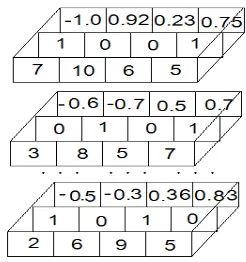
The purpose of this encoding was to find the optimal location on TCSC in terms of equations and inequalities. Therefore, the configuration of TCSC is encoded by three parameters: location, type and value (
rf
). Every individual is represented by a number of n FACTS on the string, where the n FACTS is the number of the device that needs to be analyzed in the power system, as shown in Figure 3.The first value of each string is in accordance with the location information. The value is the transmission line number where TCSC is. Each string has different value locations. In other words, it must be ensured that in one transmission line, there is only one TCSC. The second value is the type of TCSC. The stated value is the 1 value for TCSC and the 0 value for the condition without TCSC. In particular, if there is no TCSC needed on the transmission line, a value of 0 will work. The final value of
rf
declares value of the identifier of each TCSC. This value varies between -1 and +1. This real value of each TCSC is then converted according to the different types of TCSC based on the criteria. TCSC has a range betweenline
X
7 . 0
− and0.2Xline, where Xline is the reactance of the transmission line where the TCSC is
No
Yes Generate initial
Evaluate the fitness for each
Update the G, best and worst of the population
Calculate M and a for each agent
Update velocity and position
Meeting end of criterion?
Return best solution
Start
installed. Therefore,
rf
is converted into a real degree of rtcsc compensation by using the following equation:25
.
0
45
.
0
csc
=
rf
×
−
rt
(18)3.2. Population
The initial population is generated from the following parameters:
TCSC
n
: Jumlah TCSC yang ditempatkan. The number of TCSC placed.Type
n
: Type of TCSC.Location
n
: The possible location for the TCSC.Ind
n
:The number of individuals from the population.First, as shown in Figure 4, a bunch of the resultng string nTCSC was made. For each string, the first value is selected randomly from the nLocation possible locations. The second value, a type of TCSC, was obtained by taking a number randomly among selected equipments. In particular, after optimization, if no FACTS device is required for this transmission line, the second value would be set to zero. The third value of each string, containing the value of the TCSC equipment, was chosen at random between -1 and +1. The above operation was repeated as nIndtimes to obtain the whole initial population. Calculation of the whole population is shown in Figure 4.
3.3. Fitness Calculation
After encoding, each individual in the population was evaluated using the objective function. Since it related to optimization problem with the TCSC, the objective function of this problem was used as fitness function. Fitness function is the quality calculation used to compare different solution. For this purpose, the TCSC was placed on the transmission line to notice the power flow and voltage constraints. Objective function was used as the limit of TCSC placement to prevent undervoltage or overvoltage on each bus and it was able to reduce the power loss on transmission lines.
Objective function for optimizing the placement of TCSC was to minimize the power loss on transmission lines. Objective function for optimal configuration of TCSC are:
a. Active Power Loss Minimization
Minimization of active power loss (Ploss) in the transmission line:
(
)
( )∑
= =+
−
=
n j i k k ij j i j i kloss
g
V
V
V
V
P
, 1 2 2cos
2
θ
(19)where
n
is the number of transmission line,g
kis the conductance ofk
branch,V
i andV
jis thevoltage magnitude on bus i and j,
θ
ijisvoltage angle difference between bus i and j.b. Equality Constra
Power flow equation constrains is as follows:
nb
i
B
G
V
V
P
P
nj ij ij
ij ij j i Di
Gi
0
,
1
,
2
,
K
sin
cos
1=
=
+
−
−
∑
=θ
θ
(20) nb i B G V V Q Q nj ij ij
ij ij j i Di
Gi 0, 1,2,K
cos sin 1 = = ∑ + − − =
θ
θ
(21)and
Q
Dis active and reactive load from the generator,G
ijandB
ijis joint conductance andsusceptansion between bus iand bus j.
c. Inequality Constrain
Load bus voltage constraints inequality (Vi):
(
)
− − =
i
V Vi
1 exp
05 . 1 95 . 0
µ
for V etcV if
i i 1.05 95
.
0 ≤ ≤
(22)
Inequality constraints of switchable reactive power compensation (
Q
ci), inequalityconstraints of reactive power generation (
Q
Gi), inequality constraints of transformers tapsettings (
T
i), and inequality constraints of transmission line flow (Sli)stated using equations (23), (24), (25), and (26) respectively.nc i Q Q
Qcimin≤ ci≤ cimax, ∈ (23)
ng i Q Q
QGimin≤ Gi≤ Gimax, ∈ (24)
nt i T T
Timin≤ i≤ imin, ∈ (25)
nl i S
Sli≤ limax, ∈ (26)
where
nc
,ng
andntis number of switchable reactive power sources, generators and transformers.To evaluate the optimization objective function on the placement of TCSC, the best and worst fitness is calculated at each iteration as follows:
) ( min ) (
) , 1
( fit t
t
best j
N j∈ K
= (27)
) ( max )
(
) , 1
( fit t
t
worst j
N j∈ K
= (28)
wherefitj(t)is fitness in the jth agent at t time, best
( )
t and worst( )
t is the best fitness of all agents (the minimum) and worst (the maximum) fitness of all agents.d. Calculation of the Gravitational Constant
To update the G gravitational constant in accordance with population fitness of the best agents (minimum) and worst (maximum) using equation (10).
e. The Calculation of Inertia and Gravitational Mass
To calculate the value of inertial mass (M) for each agent, equations (11) and (12).
f. Calculation of the Total Force
In this step, the total force acting on the agent
i
(
F
id( )
t
)
, equations (13) and (14).g. Calculation of Acceleration and Velocity
Acceleration of
( )
a
id( )
t
and velocity of( )
v
( )
t
di from the agent
i
att
time in dth dimensions is calculated with the laws of gravity and the laws of motion, equation (15) and (16).h. Position Agent Updating
i. Repetition
In this step, the steps from c to h are repeated until the iterations reach the criterion. At the end of the iteration, the algorithm returns the value associated with the position of the agent on a particular dimension. This value is the global solution of optimization problems as well.The GSA algorithm, used to determine the optimal placement of TCSC locations and ratings, are shown in Figure 5.
4. Results and Discussion
4.1. Data of 500kV Java-Bali Power System
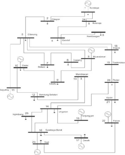
500 kV Java-Bali Power System is an interconnection system that delivers the power to customers in various areas in Java and Bali. Power is supplied from the electric power produced from various sources hydroelectric power (found in plants and SagulingCirata), steam power plant (located on the Suralaya, TanjungJati, and Paiton power plants) and steam gas power plants (consisted of Grati, Muaratawar and Gresik power plant). The single line diagram of power system can be seen in Figure 6.This study used MVA base of 1000 MVA and kV base of 500 kV as the base of 500 kV Java-Bali Power System.
Figure 5. Flowchart placement of TCSC location and optimal rating using the GSA
Figure 6. Single line diagram of 500 kV Java-Bali power system
Figure 7. Voltage profile before optimization using TCSC
0.8 0.85 0.9 0.95 1 1.05
1 2 3 4 5 6 7 8 9 10 11 12 13 14 15 16 17 18 19 20 21 22 23 24 25
V
o
lt
a
g
e
(
p
u
)
4.2. Discussion
4.2.1. Results of Load Flow before Using TCSC Optimation
To know the initial conditions of 500 Java-Bali Power System before optimization using TCSC, the load flow analysis was performed using the Newton Rapson method. The results are shown in Figures 7 and 8.
0 100 200 300 400 500 600 1-2
1-24 2-5 3-4 4-18 5-7 85- 5-11 6-7 6-8 8-9 9-10
10 -1 1 11 -1 2 12 -1 3 13 -1 4 14 -1 5 14 -1 6 14 -2 0 16 -1 7 16 -2 3 18 -5 18 -1 9 19 -2 0 20 -2 1 21 -2 2 22 -2 3 24 -4 25 -1 4 25 -1 6 P o w er l o ss
Number of line
Real power loss (MW) Reactive power loss (MVAR)
Figure 8. The power loss in transmission line before optimization using TCSC
Table 1. Parameters on the GSA
No Parameter Value
1 Population number 100
2 Iteration number 100
3 Bus number 25
4 Line number 30
In Figure 7, it shows that the variation voltage of 500kV Java-Bali Power System is in the range of 0874 to 1.020 pupu. The highest voltage occurs at bus 1 (Suralaya), namely 1.020 pu and the lowest voltage is found on the bus 20 (Pedan). From the same figure, it also shows that there are eight buses having a voltage outside the range of 0.95 ± 1.05 pu, they are: bus 12 (South London) = 0.948 pu, bus 13 (Mandiracan) = 0.911 pu, bus 14 (Ungaran) = 0.907 pu, bus 19 (Tasikmalaya) = 0.875 pu, bus 20 (Pedan) = 0.874 pu, bus 21 (Karachi) = 0.902 pu, bus 24 (Balaraja) = 0.982 pu and bus 25 (Ngimbang) = 0.946 pu.
In this Figure 8, it shows that the load flow results obtained prior to optimization using TCSC loss are of 297.607 MW of active power and reactive power losses amounting to 2926.825 MVAr with power from a power supply for 10658.607 MW of active power and reactive power generation amounting to 7338.924 MVAR. Losses of active power and reactive power was greatest in the 13-14 line for 60.593 MW and 561.663 MVAR, whereas the loss of active power and reactive power occurs at least 3-4 lines of 0.069 MW and 0.775 MVAR.
4.2.2. Load Flow Results after Optimization using the TCSC
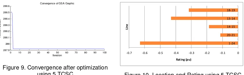
Parameters used were GSA methods to determine optimal placement of TCSC locations and ratings on Java-Bali power system shown in Table 1. The results of the convergence curve after optimization using 5 TCSC is shown in Figures 9 and 10.
0 10 20 30 40 50 60 70 80 90 100 287.9 288 288.1 288.2 288.3 288.4 288.5 288.6
Convergence of GSA Graphic
Iteration F it n e s s F u n c ti o n
Figure 9. Convergence after optimization
using 5 TCSC Figure 10. Location and Rating using 5 TCSC
Figure 9 shows that the convergence characteristics after optimization using 5 TCSC is capable of producing the active power losses in transmission lines over the minimum, when compared with the results for load flow before optimization TCSC 287.926 MW and 2355.027 MVAR.
In Figure 10, it shows that the greatest location and rating 5 TCSC on transmission system line of 500 kV Java-Bali Power System are at 1-24 lines of pu -0.6302 and the smallest rating capacity occurs in 20-21 lines of -0.1146 pu. The results of the convergence curve after optimization using 10 TCSC is shown in Figures 11 and 12.
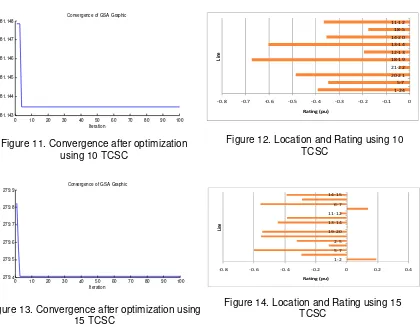
Figure 11 shows that the convergence characteristics after optimization using 10 TCSC is capable of producing the active power losses in transmission lines over the minimum, when compared with the results of optimization using load flow before TCSC of 281.143 MW and 2023.241 MVAR.
In Figure 12, it shows that the location and the rating of 10 TCSC on transmission lines of 500 kV Java-Bali Power System was greatest at 18-19 with -0.6746 and the smallest rating occurs in 21-22 lines of -0.0477 pu. The results of the convergence curve after optimization using 15 TCSC is shown in Figures 13 and 14.
0 10 20 30 40 50 60 70 80 90 100 281.143
281.144 281.145 281.146 281.147 281.148
Convergence of GSA Graphic
Iteration
F
it
n
e
s
s
F
u
n
c
ti
o
n
Figure 11. Convergence after optimization using 10 TCSC
Figure 12. Location and Rating using 10 TCSC
0 10 20 30 40 50 60 70 80 90 100 279.4
279.5 279.6 279.7 279.8 279.9
Convergence of GSA Graphic
Iteration
F
it
n
e
s
s
F
u
n
c
ti
o
n
Figure 13. Convergence after optimization using 15 TCSC
Figure 14. Location and Rating using 15 TCSC
Figure 13 shows that the convergence characteristics after optimization using 15 TCSC is capable of producing the active power losses in transmission lines over the minimum, when compared with the results of optimization using load flow before TCSC 2082.203 MW and 279.405MVAR.
In Figure 14, it shows that the location and the rating system 15 TCSC on transmission lines of 500 kV Java-Bali Power System was greatest at 1-2 at 0.1885 pu and the capacity of the smallest rating occurs in 11-12 lines of -0.0447 pu.
To keep the voltage at each bus in a span of 0.95 ± 1.05 pu, and the power flowing in each line is smaller than the maximum power, it is necessary to compensate by using TCSC on Java Bali transmission line optimization with the results shown in Figures 15 and 16.
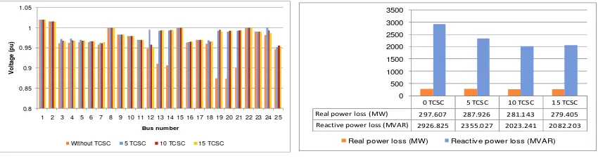
Figure 15 shows the voltage variation of 500 kVJava - Bali power system after optimization using 5 TCSC, 10 TCSC and 15 TCSC. It is in the range of 0.95+1.05 pu. The highest voltage occurs at bus 1(Suralaya) of 1.020 pu and the lowest voltage is found on the bus 25 (Ngimbang) of 0.952 pu.
In Figure 16, it shows that the total loss of active and reactive power occuring in 500 kV Java Bali power systems after optimization using 5 TCSC, 10 TCSC and 15 TCSC is
-0.8 -0.7 -0.6 -0.5 -0.4 -0.3 -0.2 -0.1 0
1-24 5-7 20-21 21-22 18-19 12-13 13-14 14-20 18-5 11-12
Rating (pu)
L
in
e
-0.8 -0.6 -0.4 -0.2 0 0.2 0.4
1-2 5-7 2-5 19-20 13-14 11-12 6-7 14-15
Rating (pu)
L
in
decreasing. The smallest active power losses occurs in the optimization of 15 TCSC at 279.405 MW, but the smallest reactive power losses is in the optimization using 10 TCSC for 2023.241 MVAR.
0.8 0.85 0.9 0.95 1 1.05
1 2 3 4 5 6 7 8 9 10 11 12 13 14 15 16 17 18 19 20 21 22 23 24 25
V
o
lt
a
g
e
(
p
u
)
Bus number
Without TCSC 5 TCSC 10 TCSC 15 TCSC
Figure 15. Comparison of the voltage profile after optimization using 5TCSC, 10TCSC, 15
with no TCSC
Figure 16. Comparison of power loss line after optimization using 5 TCSC, TCSC 10, 15
TCSC and before using TCSC
5. Conclusion
In this paper, the proposed GSA method was used to determine the location and rating of TCSC. Test results using the 500 kVJava-Bali Power System showed that the optimal placement location of TCSC rating using this GSA method could reduce the active power and reactive power losses on the line of 500 kV Java-Bali system as well as improve the value of the voltage to stay in standard limit of 0.95 ±1.05 pu. Then, load flow results after optimization using theTCSC with the GSA methods were compared by using load flow results before optimization using TCSC. The simulation results at 150 kV power generations Java-Bali showed that the GSA method was used to determine the optimal location and rating of TCSC.
References
[1] Imam Robandi. Desain Sistem Tenaga Modern.Andi. 2006.
[2] Indar Chaerah Gunadin, Muhammad Abdillah, Adi Soeprijanto, Ontoseno Penangsang. Steady-State
Stability Assessment Using NeuralNetwork based on Network Equivalent. TELKOMNIKA Indonesian
Journal of Electrical Engineering. 2011; 9(3): 412-422.
[3] Narain G. Hingorani, Laszlo Gyugyi, Mohamed E El-Hawary. Understanding FACTS Concepts and Technology of Flexible AC Transmission Systems.John Wiley & Sons, Inc. 2000.
[4] Xiao-Ping Zhang, Christian Rehtanz, Bikash Pal. Flexible AC Transmission Systems: Modelling and Control.Springer. 2005.
[5] KR Padiyar. FACTS Controllers in Power Transmission and Distribution.New Age International Publishers. 2007.
[6] MA Abido. Power System Stability Enhancement Using Facts Cotrollers: a Review.The Arabian
Journal for Science and Engineering. 2009;34.
[7] Lakshmi Ravi, Vaidyanathan R, Shishir Kumar D, Prathika Appaiah, S.G. Bharathi Dasan.Optimal
Power Flow with Hybrid Distributed Generatorsand Unified Controller.TELKOMNIKA Indonesian
Journal of Electrical Engineering. 2012; 10(3): 409-421.
[8] HO Bansal, HP Agrawal, S Tiwana, AR Singal, L Shrivastava. Optimal Location of Facts Devices to
Control Reactive Power.International Journal of Engineering Science and Technology. 2010; 2(6):
1556-1560.
[9] Ch Rambabu, YP Cbulesu, Ch Saibabu. Improvement of Voltage Profile and Reduce Power System
Losses by using Multi Type Facts Devices.International Journal of Computer Application. 2011; 13(2).
[10] SK Tsoa, J Liangb, XX Zhoub. Coordination of TCSC and SVC for Improvement of Power System
Performance with NN-based Parameter Adaptation. Electrical Power and Energy Systems. 1999;
235–244.
[11] S Jaganathan, S Palaniswami, G Maharaja vignesh, R Mithunraj. Applications of Amulti Objective
Optimization to Reactive Power Planning Problem using Ant Colony Algorithm.European Journal of
Scientific Research. 2011; 51(2): 241-253.
[12] R Mohamad Idris, A Khairuddin, MW Mustafa. Optimal Allocation of Facts Devices in Deregulated
Electricity Market Using Bees algorithm.WSEAS Transactions on Power Systems. 2010; 5.
0 TCSC 5 TCSC 10 TCSC 15 TCSC Real power loss (MW) 297.607 287.926 281.143 279.405 Reactive power loss (MVAR) 2926.825 2355.027 2023.241 2082.203
0 500 1000 1500 2000 2500 3000 3500
[13] MM Farsangi, H Nezamabadi-pour. Differential Evolutionary Algorithm For Allocation of SVC in a
Power System.International Journal technical and Physical Problems of Engineering (IJIPE). 2009.
[14] LJ Cai, I Erlich. Optimal Choice and Allocation of FACTS Devices using Genetic Algorithms. Proc. on
Twelfth Intelligent Systems Application to Power Systems Conference. 2003; 1-6.
[15] Rony Seto Wibowo, Naoto Yorino, Mehdi Eghbal, Yosshifumi Zoka, Yutaka Sasaki. Facts Devices
allocation with Control Coordination Considering Congestion Relief and Voltage Stability.IEEE
Transactions on Power Systems. 2011.
[16] Siti Amely Jumaat, Ismail Musirin, Muhammad Mutadha Othman, and Hazlie Mokhlis.Optimal
Location and Sizing of SVC Using Particle Swarm Optimization Technique.First International Conference on Informatics and Computational Intelligence (ICI). 2011; 312-317.
[17] Reza Sirjani, Azah Mohamed. Improved Harmony Search Algorithm for Optimal Placement and
Sizing of Static Var Compensators in Power Systems.First International Conference on Informatics and Computational Intelligence (ICI). 2011; 295-300.
[18] E Rashedi, H Nezamabadi-pour, S Saryazdi. GSA: A Gravitational Search Algorithm.Information
Sciences.2009;179: 2232-2248.
[19] Budi Santosa, Paul Willy. Metoda Metaheuristik Konsep dan Implementasi.Penerbit Guna Widya. 2011.
[20] Esmat Rashedi, Hossien Nezamabadi-pour, Saeid Saryazdi, Malihe M. Farsangi. Allocation of Static
Var Compensator Usin Gravitational Search Algorithm.First Joint Congress on Fuzzy and Intelligent Systems Ferdowsi University of Mashhad.2007;29-31.
[21] SS Duman, U Güvenç, N Yörükeren. Gravitational Search Algorithm for Economic Dispatch with
Valve-point Effects.International Review of Electrical Engineering. 2005;5(6): 2890-2895.
[22] Purwoharjono, Ontoseno Penangsang, Muhammad Abdillah, Adi Soeprijanto.Voltage Control on
Java-Bali 500kV Electrical Power System for Reducing Power Losses Using Gravitational Search Algorithm.International Conference on Informatics and Computational Intelligence(ICI). 2011; 11-17. [23] Serhat Duman, Yusuf Sonmez, Ugur Guvenc, dan Nuran Yorukeren. Application of Gravitational