Evaluation of Foot Kinematic Structure by the Order of Bones' and Joints' Edges.

International Journal of Modelling and Simulation, Vol. 31, No. 2, 2011

EVALUATION OF FOOT KINEMATIC

STRUCTURE BY THE ORDER OF

BONES’ VERTICES AND JOINTS’ EDGES

Ahmad Y.B. Hashim,

∗

Noor A.A. Osman,

∗∗

Wan A.B.W. Abas,

∗∗

and Lydia A. Latif

∗∗∗

Abstract

A number of distinct digital images can be formed if human foot is viewed as kinematic structure and later being converted into graphs. The synthetic images portray foot in shapes that are different from actual photographs or radiographs. The images exhibit the adjacency of bones, the incidence among bones and joints, and their paths. This study is done to find ways to represent foot in a different fashion and therefore computationally viable. The foot skeleton is studied and its structural kinematic representation is developed. This representation is later transformed into a graph. The kinematic structure is used to study the foot’s structure for engineering design viewpoints, whereas the graph is used to develop synthetic images so that foot conditions could be evaluated through pixels. This paper discusses and interprets foot conditions and anomalies. The method proposed is a one-dimensional mathematical model that is applicable in evaluating foot conditions.

Key Words

Foot, graph, kinematic structure, synthetic image

1. Introduction

Studies on human foot are not new. There are studies that look into human foot evolution [1], compare bipedal standing to ape’s [2], and discuss the process for diagnosis of foot and ankle pain [3]. Works that analyse foot kinematic structure, however, have not been found.

Within this paper, the authors propose ways to inspect human foot that employs kinematic structural and graph representations, and images derived from the developed graph. The paper discusses the arrangement of bones and

∗_{Department of Robotics and Automation, Faculty of} Manu-facturing Engineering, Universiti Teknikal Malaysia Melaka, Hang Tuah Jaya, 76100 Melaka, Malaysia; e-mail: yusairi@ utem.edu.my; ayb1@hotmail.com

∗∗_{Department of Biomedical Engineering, Faculty of} Engineer-ing, University of Malaya, Kuala Lumpur, Malaysia, e-mail: azuan@um.edu.my; {drazuan, drirwan1}@gmail.com

∗∗∗_{Department of Rehabilitation Medicine, Faculty of Medicine,} University of Malaya, Kuala Lumpur, Malaysia; e-mail: lydialatif@um.edu.my; lydialatif@yahoo.com

Recommended by Prof. A. Houshyar

(DOI: 10.2316/Journal.205.2011.2.205-5239)

how they are represented in kinematic structure and graph, the development of algebraic representations and how they are transformed into synthetic images.

Therefore, the objectives of this work are to: identify bones and joints, design structural kinematics and graph representations, develop computational models, and assess the models through exclusive cases.

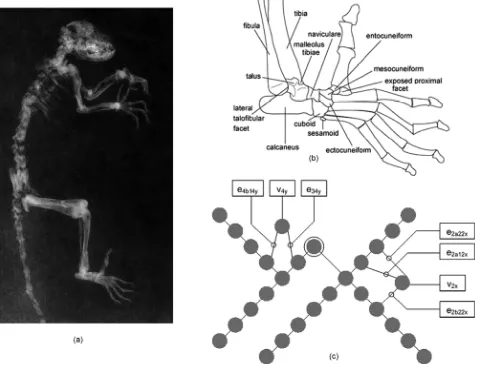
1.1 Background

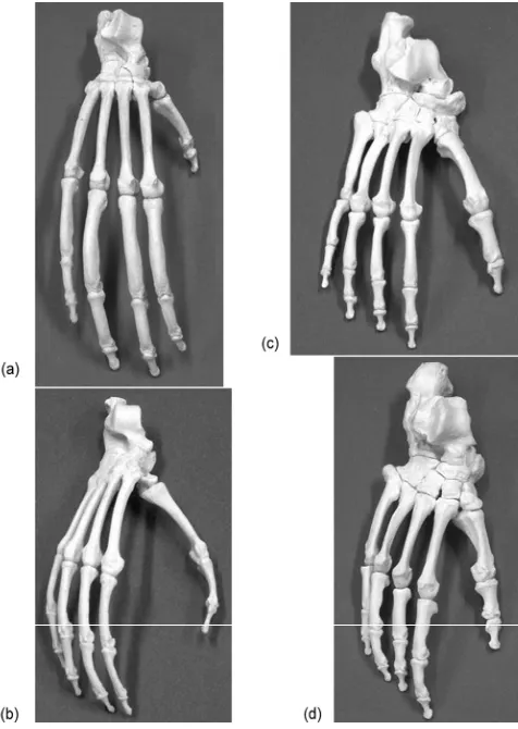
Human foot is of the plantigrade form. Figure 1(c) shows its skeleton. Its bottom is called the sole and the area behind the toe is called the ball. Major human foot bones can be identified as the phalanges – the bones in the toes, the metatarsals – the bones in the middle of the foot, the cuneiforms – the bones in the middle of the foot, actually three of them towards the centre of the foot, the cuboid – the bone adjacent to the cuneiforms on the outside of the foot, the navicular – the bone behind the cuneiforms, the talus – the ankle bone behind the navicular, and the calca-neus – the heel bone under the talus and behind the cuboid. Among primates, they share common traits. Some of the traits are the fingers with nail instead of claws, increased thumb mobility, and grasping feet [4]. In addi-tion, they have five digits on the fore and hind limbs with opposable thumbs and big toes [5].

Figure 2, e.g., exhibits selected Hominidae primates (Orangutan, Chimpanzee, and Gorilla) and a Hylobatidae primate (Siamang) skeleton feet. The five digits on the fore and hind limbs with opposable thumbs and big toes are obvious. In fact, their grasping feet are clearly shown through the thumb assembly. Siamang has the longest thumb while the Orangutan has the shortest. A human being does not possess the grasping feet capability due to unopposable thumbs, however, has better ambulation capability due to its plantigrade feet.

Figure 1. (a) The foot radiograph, (b) graph representation, and (c) foot skeleton.

Figure 2. Model foot skeletons of the (a) orangutan, (b) siamang, (c) chimpanzee, and (d) gorilla.

2. Method

2.1 Identification of Bones and Joints

Mechanical structures can alternatively be designed with the aid of graphs [6]. Before a graph is created, a kinematic structure must first be developed. Therefore, Fig. 1(b) shows the proposed outlook of foot represented by a graph. It is derived from the kinematic structure shown in Fig. 3. Talus, navicular, calcaneus, and phalanx in Fig. 1(a) are represented as vertices in Fig. 1(b). Similarly, phalanges in Fig. 1(c) are represented as vertices in Fig. 1(b).

2.2 Design of Kinematic Structural and Graph Representations

2.2.1 Kinematic Structural Representation

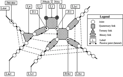
The bones and joints are identified by inspecting the skele-ton shown in Fig. 1(c). They are then assigned as links and joints in the kinematic structure shown in Fig. 3. Kinematic structure is an approach based on an abstract representation. It contains the essential information about which link is connected to which other links by what types of joints. It can be simplified by a graph. The graphs can be enumerated using combinatorial analysis and computer algorithm [6].

In Fig. 3, L1 is connected to L2 as well as L3 by

revolute joints J12 and J13, respectively. The L1 and L2

are quaternary links,L4is ternary link, andL3is a binary

Figure 3. Link and joint labelling for the kinematic structural representation. The legend shows, e.g., a shaded triangle that translates into a ternary link. It has three possible connection points, the circles that translate into revolute joints. The passive joints act laterally, in which their significance in modelling of the architecture are neglected.

two links, one on the right-hand side and another on the opposite, are labelled as “2” and “3”, respectively. Branches after the second layer are labelled with an al-phabet in addition to number arrangement, so thatL2a1is

located on the right-hand side, the first link afterL2. The

successive links are labelled as L2a1, L2a2, L2a3, L2a4. A

couple of dark-shaded circles represent fibula and tibia.

2.2.2 Graph Representation

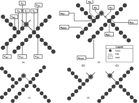
There is similarity in overall build but differs in the profiles that define a link and a joint, where in graphs, circles represent vertices and lines represent edges. Moreover, a vertex is equivalent to a link and an edge to a joint. Figure 4 shows the graph derived from Fig. 3. The subscripts on labels for vertices and edges maintain. Figure 4 exhibits 26 vertices and 25 edges that form a labelled and rooted tree. Row one in Table 1 describes that the subsequent v2

andv3are both connected formerly to v1, which happens

to be the root of the tree. We have v1≺v2 and v1≺v3.

An edge comes in between vertices. Row one in Table 1 explains thate12lies in betweenv1andv2, wherease13lies

in betweenv1andv3. In Fig. 4(d), there are two subgraphs

G1andG2. These are two significant groups that branch

off but share the root. They are divided into group 1, group 2, and group 3.

2.3 Development of the Computational Model

2.3.1 Vertex-Edge Adjacency, Incidence, Path

A graph consists of vertices and edges [7]. In this work, vertex represents bone, edge-joint. In Fig. 1(b), verticesv

are shown as circles, edgeseas the connecting lines. There are a number of paths that have originated from the root – talus, v1. Each label for vertex and edge portrays the

location of joint or bone, e.g., v2a1 precedesv2,e22a1is in

betweenv2 andv2a1.

The degree of vertex depends on the number of edges within a graph. In fact, it is straightforward that the degree of a vertex is the sum of a particular column or row in the adjacency matrix. The total number of vertices is the number of subsequent verticesNs added to one or Nv= ΣNs+ 1, and the number of edges –

Ne=Nv−1.

The vertex-to-vertex matrix facilitates adjacency of the vertices. It is defined in (1). It is anNv×Nv symmet-ric having zero diagonal elements. Similarly, (2) defines incidence matrix that outlines vertices and edges. In (3), it defines the path – the matrix that stores information about all paths emanated from the root. It is a Ne×(Nv−1) excluding the root.

Figure 4. Vertex and edge labelling for graph architecture. Note that the circles translate into vertices, in which vertices are actually links in the kinematic structural representation. One has to craft the kinematic structural representation of a mechanism before graphs can be developed. Labels for (a) vertex and (b) edge are shown. The general graphs (c) and (d) the subgraphs are shown.

Table 1

Vertex and Edge Labelling

Groups Vertex Edge Consequential Bone

1 v1, v2, v3, v4 e12, e13, e34 Talus, calcaneus, navicular, cuboid

2 v2, v2a1, v2a2, v2a3, v2a4 e22a1, e2a12a2, e2a22a3, e2a32a4

Cuneiforms, metatarsals, phalanges

v2, v2b1, v2b2, v2b3, v2b4, v2b5 e22b1, e2b12b2, e2b22b3, e2b32b4, e2b42b5

v2, v2c1, v2c2, v2c3, v2c4, v2c5 e22c1, e2c12c2, e2c22c3, e2c32c4, e2c42c5

3 v4, v4a1, v4a2, v4a3, v4a4 e44a1, e4a14a2, e4a24a3, e4a34a4 Cuboid, metatarsals,

v4, v4b1, v4b2, v4b3, v4b4 e44b1, e4b14b2, e4b24b3, e4b34b4 Phalanges

This arrangement relates every component to its associated bone. In addition, it provides easy access to refer for the number of particular bones and formal labels in graphs.

the sequence is a path if it has distinct vertices and edges, or a trail if the edges are unique [6]. We have

A=

⎧

⎪ ⎪ ⎪ ⎪ ⎪ ⎪ ⎨

⎪ ⎪ ⎪ ⎪ ⎪ ⎪ ⎩

[ai,j, Nv×Nv]

⎛

⎝ai,j=

⎧

⎨

⎩

1 ifvi is adjacent tovj 0 otherwise andi=j

⎞

⎠; v∈V ⎫

⎪ ⎪ ⎪ ⎪ ⎪ ⎪ ⎬

⎪ ⎪ ⎪ ⎪ ⎪ ⎪ ⎭

(1)

B=

2.3.2 Synthetic Image

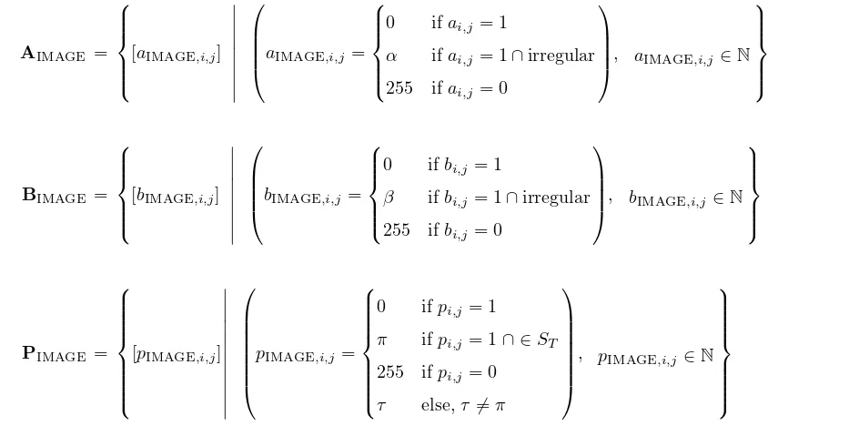
It is difficult to visualize solutions to (1), (2), and (3) because they appear in large matrices with digits 0 and 1 only. However, every solution holds a unique pattern. The patterns depend on the algorithms presented in (1)–(3). The information contained in them explains foot architecture based on the arrangement of bones and joints. To make easy reading of the patterns, (1)–(3) are amended

AIMAGE =

3. Model Assessment

3.1 Foot Model

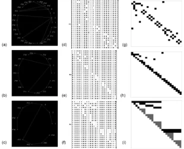
Taking Fig. 1 as model, (1) is used to solve for the vertex adjacency, (2) for the vertex–edge incidence, and (3) for the paths. The solutions are shown in Fig. 5(d)–(f). It is noticed that they display as large matrices. In addition, Fig. 5(a)–(c) shows the computer plots for graph, sub-graphsG1andG2. Lastly, Fig. 5(g)–(i) depicts

character-istic images for vertex adjacency, vertex–edge, and paths, respectively. They are generated following (4)–(6). The five grey triangles in the path image represent the digits.

into (4)–(6). Outputs from (4) to (6) are characteristic images in greyscale.

A greyscale image has the scale of natural numbers that begins from 0 and ends at 255. The digit 0 characterizes a pure black, whereas 255 a pure white. In (4), elements

α exist if bone irregularities are found. Similarly, in (5), elementsβexist if bones and joints irregularities are found. In (6), however, elements π exist if they are within the sequence of trails:

The adjacency matrix is 26×26. The element a12= 1

indicates v2 is adjacent to v1, where talus borders

calca-neus. Thea23,a24, anda25 exhibit their adjacency to one

common vertex in which vertices v2a1, v2b1, and v2c1 are

adjacent tov2. The zero diagonal implies that none of the

vertices mirror to themselves. Its image has a discrete “←” shape.

Figure 5. (a) The graph plots for human foot, (b) subgraphG1, (c) subgraphG2, (d) adjacency matrix, (e) incidence matrix,

(f) path matrix. The characteristic images: (g) adjacency image, (h) incidence image, and (i) path image.

Figure 6. The description of grey triangles with respect to actual bones representation.

The vertex–edge path matrix is 25×25. Its signifi-cance is shown by five grey triangles in its image. These triangles depict the foot’s five digits shown in Fig. 6. The first three triangles belong to the vertex–edge group 2, and the remaining two triangles belong to the vertex–edge group 3. It explains the possible paths from the root until

vj+1.

The sequence ofST1begins frome22a1and terminates

at v2a4. It is within the first grey triangle. The sequence

of SP1, however, begins from v2 and terminates at v2a4.

All paths contain v2. This distinguishes SP from ST.

A trail can only have unique elements. In fact, all trails are represented by the grey triangles. Nevertheless, the sequence of all walks begins from the rootv1and terminates

on last vertex of respective paths. Therefore, the set of phalanges in Fig. 5(f) has submatrixST5 that is visible in

G2and is shown in (7) whereπ= 128:

submatrix (P:⇔_PIMAGE,22,25,22,25) =

S_T5

⎡

⎢ ⎢ ⎢ ⎢ ⎢ ⎢ ⎢ ⎢ ⎣

128 128 128 128 255 128 128 128 255 255 128 128 255 255 255 128

⎤

⎥ ⎥ ⎥ ⎥ ⎥ ⎥ ⎥ ⎥ ⎦

(7)

3.2 Simulation

Supposev2b5 is absent. It is known that v2b5 is phalanx

and its edge is e2b42b5 from Table 1. If v2b5 is absent so

woulde2b42b5. It is evident that (7), with the absence of

phalanx denoted asα= 129, develops into (9):

ST2=e22b1, v2b1, e2b12b2, v2b2, e2b22b3, v2b3, e2b32b4, v2b4

(8)

submatrix (A:⇔AIMAGE,11,12,11,12) =

v2b5

⎡

⎣

255 129

129 255

⎤

⎦

Figure 7. (a) The foot complication due to diabetes, (b) the graph plot, (c) the adjacency matrix, and (d) the adjacency image.

Supposev4a1is absent. Consequently, non-appearance

ofe44a1 ande4a14a2. Non-existence of the vertex is shown

in (10). The pixels within the submatrix are isolated from

G. This indicates connection lost becauseST4is no longer

a member ofSP4: 129 255 255 129 0 255 255 255 255 129 255 255

⎤

Suppose v2 is absent. Absence of calcaneus causes

a large part of the foot system to uncouple, so that

SP1=ST1, SP2=ST2, SP3=ST3, ∩3i=1SPi= Ø, and

∩3

i=1SWi={v1}. These phenomena are seen in G2. In

(11), the four pairs of pixels α= 129 shows that a large portion of the components is uncoupled:

submatrix (A:⇔_AIMAGE,1,5,1,5) =

255 129 255 255 255 129 255 129 129 129 255 129 255 255 255 255 129 255 255 255 255 129 255 255 255

⎤

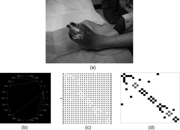
3.3 Diabetic Foot

By inspection, foot complication due to diabetes shown in Fig. 7(a) has lost some phalanges. Alternatively,

Table 2

Technical Specifications for Diabetic Foot

Specification Information

Fig. 7(b)–(d) reports this condition through a graph, ad-jacency matrix, and adad-jacency image, respectively. The adjacency matrix depicts lost phalanges as zeros. The α

value is assigned to the four pairs lost vertices to exhibit irregularity.

Table 2 summarizes the condition that lists specifi-cations based on the bone group and type, the lost ver-tices and edges, and the assigned greyscale to show the irregularities on the adjacency characteristic image.

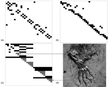
3.4 Primate Foot –Darwinius masillae

Figure 8. Darwinius masillae, a new genus and species: (a) the complete fossil, (b) the skeleton foot illustration, and (c) the proposed graph.

Table 3

Vertex and Edge Labelling and Their Associated Bones that elong toDarwinius masillae

Groups Vertex Edge Consequential Bone

1 v1, v2, v3, v4, v4y e12, e13, e34, e34y Talus, calcaneus, navicular, cuboid, sesamoid

2

v2, v2x, v2a1, v2a2, v2a3, v2a4 e22a1, e2a12x, e2a12a2, e2a22a3, e2a22x, e2a32a4 Entocuneiform, mesocunieform,

v2, v2b1, v2b2, v2b3, v2b4, v2b5 e22b1, e2b12b2, e2b22b3, e2b22x, e2b32b4, e2b42b5 endocunieform, exposed proximal

v2, v2c1, v2c2, v2c3, v2c4, v2c5 e22c1, e2c12c2, e2c22c3, e2c32c4, e2c42c5 facet, metatarsals, phalanges

3 v4, v4a1, v4a2, v4a2, v4a3, v4a4 e44a1, e4a14a2, e4a24a3, e4a34a4 Metatarsals, phalanges

v4, v4b1, v4b2, v4b3, v4b4 e44b1, e4b14y, e4b14b2, e4b24b3, e4b34b4

The adjacency matrix is 28×28. In Fig. 9(a), its adjacency has the “←” shape. It is similar to human’s, but there is a variant due tov2x andv2y. This is further

explained in Fig. 10 where the profile for bones adjacency of human and Dm is compared. The incidence matrix size is 28×30. In Fig. 9(b), its incidence has the “ ” shape

and is also similar to human’s, but there is a variant due toe2a12x,e2a22x,v2x,e4b14y,e34y, andv2y.

The path matrix is 30×27. The path image in Fig. 9(c) shows five grey triangles. The image, however, has a smaller first grey triangle. There is an isolation line that sets apart the first and second triangles due to e2a12x,

Figure 9. Characteristic images ofDarwinius masillae: (a) adjacency, (b) incidence, (c) path, and (d) Dm’s foot.

Figure 10. The vertex adjacency profile for human and Dm.

e2a22x, andv2x. This line also set aside the third and fourth

triangles due toe4b14y,e34y, andv2y. The sequence of trail

ST1Dm begins from e22a2 and terminates at v2a4. This is

represented by the first triangle in the path image.

4. Discussion

The results of the examined cases lead to the conclu-sion that reporting for foot anomalies and evaluating for primate foot can be characterized by graphs, algebraic representations, and characteristic images. However, the method limits its employability to only situations that require foot analysis based on the presence, absence, or irregularities of the bones. The case of diabetic foot is the example. As to check if a species is a primate, Dm for example, its characteristic images bear a resemblance to human. In addition, the method is seen useful in plan-ning for humanoid robot design, especially their foot or hand such as the work done in [9] where human-like fin-ger mechanism is designed to have effective grasp operation.

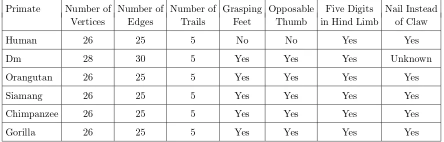
Except for human feet, primates have feet that are meant for grasping, so that Siamang, Chimpanzee, Gorilla, Orangutan, and Dm can climb trees with ease. They share a similar trait – the sequence of trailST1is the opposable

Table 4

Primate Foot Comparison Based on the Number of Vertices, Edges, Trails, and the Standard Primate Classification Criteria

Primate Number of Number of Number of Grasping Opposable Five Digits Nail Instead Vertices Edges Trails Feet Thumb in Hind Limb of Claw

Human 26 25 5 No No Yes Yes

Dm 28 30 5 Yes Yes Yes Unknown

Orangutan 26 25 5 Yes Yes Yes Yes

Siamang 26 25 5 Yes Yes Yes Yes

Chimpanzee 26 25 5 Yes Yes Yes Yes

Gorilla 26 25 5 Yes Yes Yes Yes

is seen in human, Orangutan, Siamang, Chimpanzee, and Gorilla. Dm, however, has more vertices as well as edges but the number of trails agrees to the others. Therefore, the “grasping feet” and the “opposable thumb” can become the secondary criteria in classifying primates.

5. Conclusion

In this work, the bones network is the idea shown in Fig. 2. The effects of lateral joints are disregarded. This network, however, should become different if the complex muscle interconnections are taken into account. The kinematic structure offers a formal representation of links and joints. One can easily identify and pinpoint the joints and bones through the representation. Conversely, the graph provides a simpler view than the kinematic structure. Once the graph is developed, at least three relational matrices are created. They are the adjacency, incidence, and path matrices. They explain vertex-to-vertex and vertex-to-edge relationships. It is, however, easier to read the matrices if they are converted into synthetic images. It is because their sizes are too large. Only digits “0” and “1” appear in the matrices. So, the characteristic images provide clearer views.

By manipulating the greyscale 0–255, the image can be made to exhibit, e.g., foot anomalies or foot whether it is primate. In fact, a fossil foot can be analysed and iden-tified if it belongs to the primate family. Nonetheless, the method proposed in this paper complements the standard foot examination procedures such as using radiographs or photographs. The method proposed should be useful as medium for communication among different professionals who involve directly or indirectly into foot medicine, re-search, and science. For future works, the authors suggest that the method be programmed as application software for rehabilitation medicine practitioners.

Acknowledgement

This work is funded through the Malaysian Ministry of Higher Education’s Fundamental Research Grant Scheme FRGS/2008/FKP(4)-F0069.

References

[1] R.J. Clarke & P.V. Tobias, Sterkfonein-member-2 foot bones of the oldest South-African hominid,Science,269, 1995, 521–524. [2] W.J. Wang & R.H. Crompton, Analysis of the human and ape foot during bipedal standing with implications for the evolution of the foot,Journal of Biomechanics,37, 2004, 1831–1836. [3] J.S. Newman & A.H. Newberg, Congenital tarsal coalition:

Multimodality evaluation with emphasis on CT and MR imaging, RadioGraphics,20, 2000, 321–332.

[4] C. Soligo & A.E. M¨uller, Nails and claws in primate evolution, Journal of Human Evolution,36(1), 1999, 97–114.

[5] F.W. Pough, C.M. Janis, & J.B. Heiser,Vertebrate life, Seventh Edition (Upper Saddle River, NJ: Benjamin Cummings, 2004). [6] L.-W. Tsai, Mechanism design: Enumeration of kinematic structures according to function(Boca Raton, FL: CRC Press, 2001).

[7] G. Chartrand & P. Zhang, Introduction to graph theory (New York: McGraw-Hill, 2005).

[8] J.L. Franzen, P.D. Gingerich, J. Habersetzer, J.H. Hurum, W. von Koenigswald, & B.H. Smith, Complete primate skele-ton from the Middle Eocene of Messel in Germany: Mor-phology and paleobiology, PLoS ONE, 4(5), 2009, e5723. Doi:10.1371/journal.pone.0005723.

[9] S. Yao, L. Wu, M. Ceccarelli, G. Carbone, & Z. Lu, Grasping simulation of an underactuated finger mechanism for Larm Hand, International Journal of Modelling and Simulation,30(1), 2010. Doi:10.2316/Journal.205.2010.1.205-5134.

Biographies

Ahmad Y.B. Hashim obtained

and Robotic Laboratory, Institute of Advanced Technology, Universiti Putra Malaysia from 2003 to 2004.

Noor A.A. Osman graduated

from University of Bradford, UK with a B.Eng. Hons in Mechanical Engineering, followed by M.Sc. and Ph.D. degree in Bioengineer-ing from University of Strath-clyde, United Kingdom. Azuan’s research interests are quite wide-ranging under the general um-brella of biomechanics. However, his main interests are the mea-surements of human movement, prosthetics design, the development of instrumentation for forces and joint motion, and the design of prosthetics, orthotics and orthopaedic implants. In 2004 he received BLESMA award from ISPO UK NMS in recognition of his significant contribution to the development of the prosthetic socket. He is curently the Deputy President of Society of Medical and Biological Engineering (MSMBE), affiliated organisations of International Federation for Med-ical and BiologMed-ical Engineering (IFMBE). He is also the Head of Department of Biomedical Engineering, and the Coordinator of Motion Analysis Laboratory of Faculty of Engineering, University of Malaya. He has publications in books, conference proceedings, and journals.

Wan A.B.W. Abas obtained his Bachelor of Science (Mechanical Engineering) degree in 1974 and Ph.D. (Bioengineering) degree in 1978, both from the University of Strathclyde, Glasgow, Scotland, United Kingdom. He joined the University of Malaya in 1976 as a tutor and in 1978 appointed as a lecturer at the Department of Mechanical Engineering. He was promoted to the associate profes-sor post in 1985 and the profesprofes-sor post in 1995. In 2000, he was transferred to the Department of Biomedical En-gineering which he founded. He was three times Dean of the Faculty of Engineering (1984–1999, with breaks) and first head of department of the Department of Biomedical Engineering (2001–2002). He is currently a professor in the Biomedical Engineering Department as well as President of the Malaysian Society of Medical and Biological Engi-neering (MSMBE). His research interests are in the areas of tissue mechanics, motion analysis, and tissue engineering.

Lydia A. Latif obtained her